
All advanced methods in GHEtool require an hourly load profile, which is typically not available in the early design stages. However, it is precisely in this early design and feasibility phase that concepts are decided upon and that a deeper knowledge of the geothermal potential is useful. Today we solved this by letting you create an hourly demand profile in seconds!
Advantages of having an hourly load profile
We already discussed quite a lot in the past what the advantage of having an hourly load profile is (as in our latest article here). Hourly profiles contain important information on how ‘spiky’ the heating and cooling demand of the building is and when these peaks typically occur. This makes it possible, for example, to differentiate between a building with a slow emission system (such as floor heating) or one where heating and cooling is mostly done by the air handling unit. This hourly information is therefore essential to optimise or simulate hybrid systems, or to combine active and passive cooling with the geothermal borefield.

Besides requiring this information for the more advanced methods within GHEtool, there is also the problem of simultaneity (which we discussed in our previous article) in collective systems. When multiple users are connected to a single collective borefield, the resulting peak power on the borefield is typically lower than the total sum of all peak demands. This is because not all buildings are the same and the residents have different behaviour. The percentage of the installed demand compared to the peak demand is called the simultaneity.
Due to this simultaneity, the power for which you design your borefield can sometimes be smaller, especially in larger collective systems with more than 100 units. However, for geothermal systems, not only the peak demand but also the peak duration is important. By using an hourly load profile, it is now possible to estimate this more accurately and to make the design of collective systems easier and more reliable than ever before.
In the next section we discuss the methodology behind this hourly load profile generator, after which we show you how easy it is to use in GHEtool Cloud.
Methodology
It should be clear that hourly load profiles offer far more insight in geothermal designs, but typically they are created based on dynamic simulations of the building, which require quite a lot of information, time and money. These three things are usually not available in the early stages. That is why we developed a methodology to create an hourly load profile based on just the following inputs:
- Yearly heating/cooling demand of the building(s)
- Yearly peak heating/cooling demand of the building(s)
- Installed power heating/cooling of the building(s)
- Weather profile (EPW or based on location)
!Note
The installed power can be different from the yearly peak demand. Imagine a building with a peak demand of 12 kW but with only a heat pump of 10 kW installed, or the other way around. This is especially important for collective systems with high simultaneity, since it influences the peak duration.
Heating and cooling degree days
The idea behind this method is that the heating and cooling demand is related to the outside air temperature, as in the case of heating and cooling degree days (find more information here).

- By starting with a weather file and an initial threshold temperature above which heating begins, an hourly profile is obtained. The higher values occur at the hours when the temperature is lower and therefore the difference between the temperature and the threshold is the greatest. It is at these moments that we also expect the highest peak demand. The same reasoning can be applied to the cooling demand.
- Next, this hourly profile is scaled with the yearly energy demand (which is an input) to create an hourly load that has the same yearly demand as the building.
- Finally, the peak power should be checked. If the peak power of the profile is different from the peak demand of the building, the temperature threshold is adjusted so that the heating starts earlier or later and the second step is repeated.
!Note
Imagine, for example, that in step 2 the peak heating demand in our profile is greater than the actual estimated demand. In that case we assume that heating starts too late in the season, since the demand is too concentrated, leading to high peak powers. By lowering the temperature threshold at which heating starts, the hourly profile is widened and, after rescaling, the peak powers are reduced.!Note
In this step we are still talking about the actual building demand, so the peak demand is used and not the installed power.
- Finally, it can happen that our yearly energy demand as well as our peak demand match with the profile, but that the actually installed peak power is lower. When this is the case, the peak power is limited to the installed power and the load is shifted in time. For example, if we have a peak demand of 10 kW but only an installed power of 8 kW, then 1 kW is shifted to the hour before and 1 kW to the hour after. If that hour also has a demand higher than 8 kW, the load is shifted further in time, which indirectly increases the peak duration.
!Note
It is important to note that this method will give you a good first estimate of a realistic hourly load profile, but of course this depends very much on the building itself. Factors such as comfort temperature and occupancy behaviour are not included in the described method. Therefore, this method should not be used to replace dynamic building simulations but to complement them in the early stages.
Generate hourly loads with GHEtool Cloud
In this section we briefly go over the flow of how you can create your own hourly load in GHEtool using the method described above.
Under the Thermal Demand tab, you will find a ‘create hourly load’ button. This button is only visible when you have not already uploaded an hourly load profile. Clicking it opens the following tab.

As discussed in the methodology above, we need a weather file to create this hourly profile, which can either be uploaded manually or found based on the location.
!Note
The typical meteorological year is created based on the PVGIS project, which covers the entire world and is freely available online using this link.
For both a single user and a collective system, the inputs are the same: you need an estimate of the peak power in heating and cooling, as well as an estimate of the yearly heating and cooling demand for the entire project. When you select a collective system, you have the option to enter the number of connected users to calculate the simultaneity. Otherwise, you can set the installed power to a value higher or lower than the building demand.
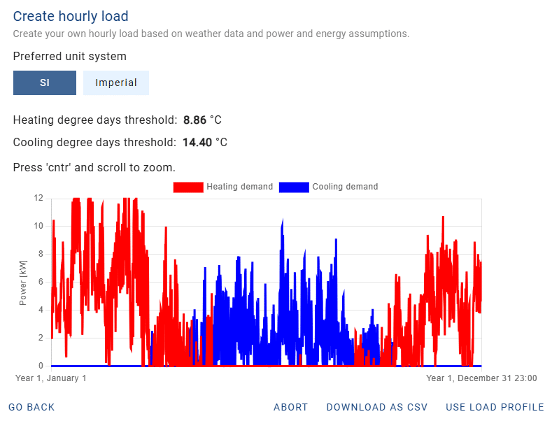
Below you can find a generated hourly load for a heating demand of 15 kW.

!Note
For your information, the heating and cooling degree thresholds are also given. This is a result of the methodology used to achieve a profile with the same peak power and yearly energy demand, and not a strict temperature setting on the thermostat. So when the figure above shows that cooling starts above 14.4°C, this simply determines when the cooling period begins, based on the peak cooling and yearly cooling demand you entered. If you think this threshold is too low, you can either increase your peak cooling demand or decrease your yearly cooling demand to raise the threshold and effectively make the cooling season shorter.
For the profile below, an installed power of 12 kW was set for the heating load. As you can see, both temperature thresholds are the same, since the building demand has not changed, but the profile looks slightly different. The peak power is shaved in winter, which leads to a longer peak duration at a lower peak power.
Conclusion
This article discussed a new but very powerful feature in GHEtool to create an hourly load profile with only a minimum of settings. The advantage is that even in the early stages, the more advanced methods of GHEtool become available, and the simultaneity of collective systems can be taken into account without relying on complicated and expensive dynamic building simulations.
References
- Watch our video explanation over on our YouTube page by clicking here.