
In the previous chapters, the concepts of pressure drop, pump power, and pump energy were introduced. In this chapter, these insights will be used to carry out our first hydraulic design in GHEtool Cloud.
Hydraulic design of the borefield
The hydraulic design of borefields goes beyond simply selecting the pipe diameter used inside the borehole. The entire horizontal design also plays an important role: what is the horizontal pipe diameter? How many bends or junctions are there? How are the boreholes connected to each other?
In the following sections, the different ways of connecting boreholes (in parallel, Tichelmann, or in series) are explained, followed by the concept of hydraulic balancing.
Horizontal connections
When there are multiple boreholes in a system, they are typically connected to a manifold in one of four different ways: direct, parallel, Tichelmann, or series. These options are explained below.
Direct
When the boreholes are connected directly to the manifold, the flow rate through each borehole is the same as the flow rate through the horizontal section. This is the most straightforward way of connecting boreholes and has the advantage of offering greater flexibility to control the different boreholes individually. In addition, it provides an extra level of safety in case something goes wrong. Since the boreholes can be disconnected individually, issues can be managed more easily.
The main disadvantage of a direct connection is that it is more expensive, as a larger manifold and more horizontal connections are required. In addition, since the flow rate is now divided over the $n$ boreholes in the system, it can be more difficult to achieve turbulent flow.
Parallel connection
For a parallel connection (also called direct return) of the boreholes, the number of horizontal connections is smaller than the number of boreholes. This means that a single horizontal connection can, for example, be connected to 2, 3, or more boreholes. This has the advantage of requiring fewer horizontal connections and welds, making the system more cost-effective. The manifold can also be smaller, due to the lower number of connections.
The disadvantages are that flexibility in control is reduced, since not every borehole can be controlled or balanced individually. This also means that when one borehole fails or leaks, the entire parallel connection is affected. In addition, since boreholes are connected in groups of n, the flow through the horizontal section is n times the flow through each borehole, which highlights the importance of proper hydraulic design of the horizontal pipe diameter.
Below, an image of the parallel connection (direct return) is shown.

The figure above shows two hydraulic “parallel” configurations. The one on the left, reverse return piping, is also called Tichelmann and will be discussed next. The one on the right is the traditional parallel connection. Although this design is simpler to implement, it does not guarantee an equal flow rate through the different boreholes. The path through borehole 1 is shorter than the one through borehole 2, resulting in lower friction losses and therefore a slightly higher flow rate. This is generally undesirable (as will be discussed below), which is why a Tichelmann connection is typically preferred.
Tichelmann connection
When the boreholes are connected in a Tichelmann configuration, they are still grouped in sets of n, resulting in a factor n fewer horizontal connections than in the case of a direct connection and an n times higher flow rate in the horizontal section. In that sense, it is very similar to the parallel connection described above, with the key difference that the return pipe has the same length for every borehole. This ensures that the pressure losses for each borehole are identical, resulting in an equal flow rate through each borehole. All other benefits of a parallel connection still apply here.
The disadvantages are again the reduced ability to control individual boreholes (although, in theory, a Tichelmann connection is always hydraulically balanced).
Series connection
A series connection is typically used when a higher flow rate through the boreholes is desired in order to improve heat transfer. By connecting boreholes in series in groups of $n$, the number of horizontal pipes is again reduced by a factor n, but now because the outlet of one borehole is directly connected to the inlet of the next. This means that the flow rate in every borehole is identical and equal to the flow in the horizontal pipes. An example of a series connection is shown below.
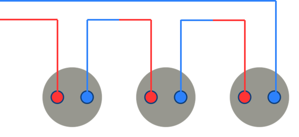
The main advantage of a series hydraulic design is that it is easier to achieve turbulent flow due to the higher flow rate per borehole. It is also relatively cost-effective, since no complex hydraulic connections are required, as in the case of a Tichelmann configuration, and fewer pipes are needed than in a direct connection. The disadvantage of a series connection is that, when one borehole has a problem, all boreholes in that group are affected. In addition, since the flow must pass through all boreholes, the pressure drop for a series connection is significantly higher than for a direct or Tichelmann design.
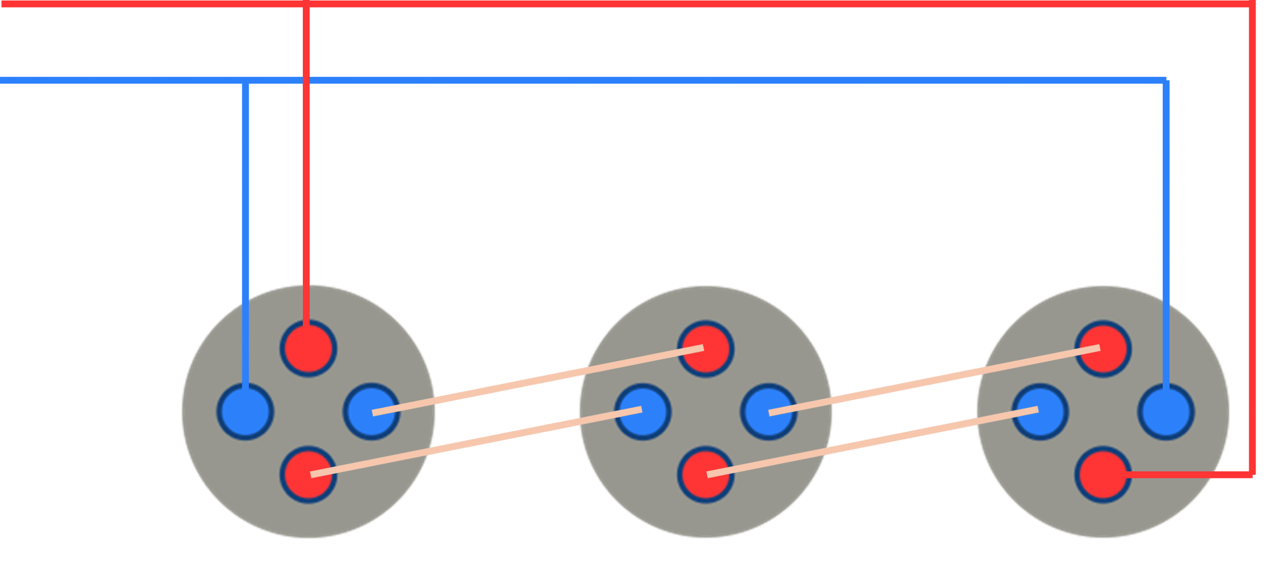
When connecting double U-tubes in series, it is common for both U-tubes to have different inlets and outlets. For example, if two boreholes are connected in series, one pair of U-tubes will have the inlet in the left borehole flowing towards the right, while the other pair will have the inlet in the right borehole flowing towards the left. This ensures better balancing of extraction and injection. This is also shown in the figure below, where the red line represents the inlet and the blue line the outlet.
Combination
Of course, it is also possible to combine different horizontal configurations, as shown in the image below.
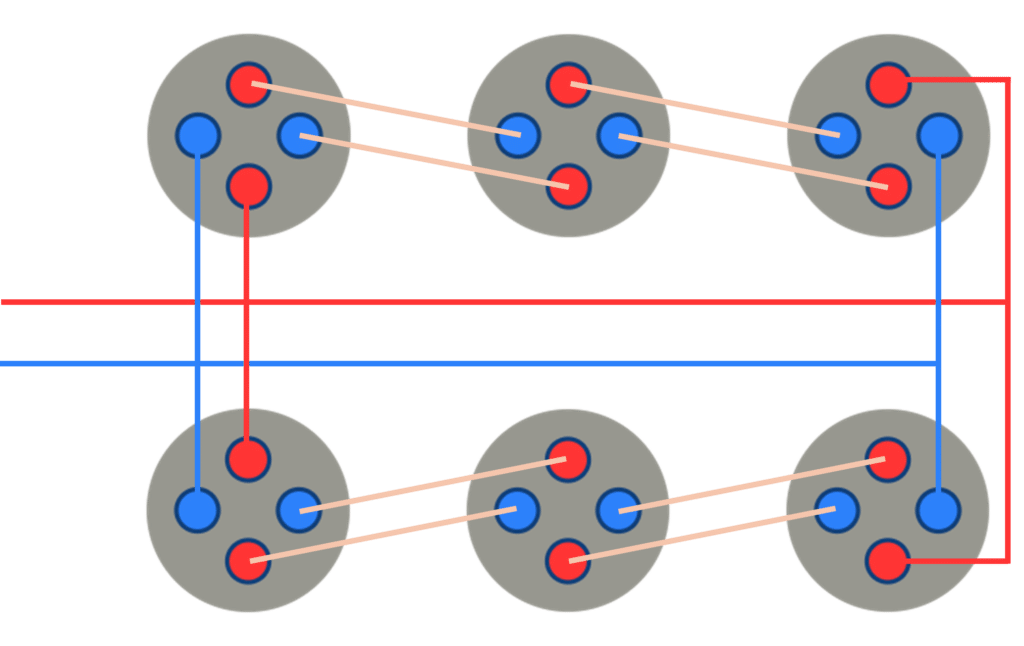
Here, the boreholes are divided into two groups of three boreholes. Within each group, the boreholes are connected in series, and the two groups are then connected in a Tichelmann configuration. Such complex designs can occur for various reasons but are often avoided due to the high risk of installation errors.
Hydraulic balancing
As mentioned in the first chapter of this part, the pressure drop along a given hydraulic path is determined by both the length of this path and all local losses (bends, junctions, etc.). In a geothermal borefield, this can vary significantly from one borehole to another, since some are closer to the manifold while others are further away. The key to calculating the overall pressure drop of such a complex system in a relatively straightforward way is the concept of hydraulic balancing.
From a thermal perspective, it is ideal for each borehole to contribute equally to the power and energy demand of the system. Therefore, the goal is to achieve the same flow rate through each borehole. This can be ensured by making the pressure drop for each borehole (i.e. each hydraulic path) identical. This is achieved by calculating (or measuring in the field) the pressure drop of the worst-case path and ensuring that all other boreholes have the same pressure drop using balancing valves.
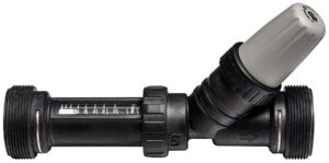
Using these valves, an additional local pressure drop can be introduced at each connection to the manifold in order to achieve hydraulic balance.
For the hydraulic design of borefields, the key is to identify the worst-case situation where the pressure drop is highest. This is typically the borehole that is furthest from the manifold, resulting in the largest horizontal pressure losses. Since all other boreholes are adjusted to have the same pressure drop, calculating a single hydraulic path is sufficient to determine the overall pressure drop of the system.
This concept of hydraulic balancing ensures that the total pressure drop, for a given design flow rate, is identical for all connections to the manifold. However, this does not mean that the friction losses and local losses are identical for each hydraulic path. Some connections will have fewer horizontal pipes and therefore require more local losses to compensate, while others will have higher horizontal pressure losses and require fewer additional local losses.
The fact that these flow or balancing valves are static (meaning that once set, they maintain the same K-value) introduces an additional complexity in the hydraulic design. The total pressure drop equation is given again below:$$\Delta P = \left(f\cdot \frac{L}{D}+\sum{K}\right)\cdot \frac{\rho v^2}{2}$$where $\Delta P$ is the pressure drop in (Pa), $f$ is the Darcy-Weisbach friction factor, $L$ and $D$ are the pipe length in (m) and pipe diameter in (m), $\rho$ is the fluid density in (kg/m³), and $v$ is the flow velocity in (m/s).
When the flow rate changes, the flow velocity $v$ also changes, affecting both local and friction losses. However, as discussed in Part 4.1, the friction factor is also a function of the flow rate (via the Reynolds number). This means that the friction losses are more strongly affected than the local losses. As a result, when operating away from the design set point of the balancing valves, the system may no longer be perfectly balanced due to the difference in how local and friction losses respond.
It should be noted that, although this effect exists, its impact on the overall system performance is generally limited. When necessary, dynamically controlled balancing valves can be used to adjust the K-value depending on the flow rate. However, these systems are significantly more expensive, both in terms of initial investment and ongoing maintenance.
Hydraulic design in GHEtool Cloud
In GHEtool, three different pressure drop contributions are considered in the hydraulic design: the part inside the borehole itself, the connections between the boreholes and the manifold, and the connection from the manifold to the technical room.
In the screenshot below, the different contributions are clearly shown.
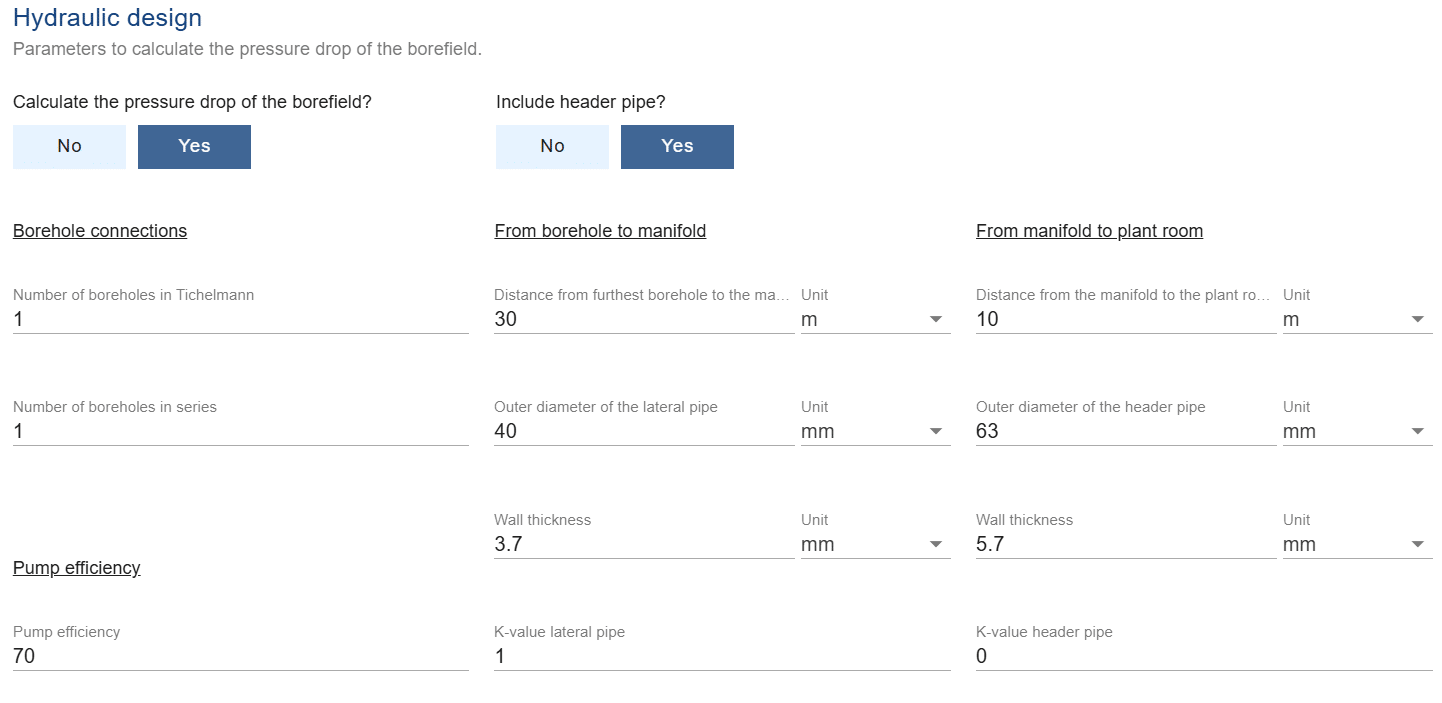
Different input parameters
For the borehole connections, a selection or combination of Tichelmann and series connections can be made. When all boreholes are connected directly to the manifold, both values are set to 1, meaning that each group contains a single borehole. For the combined case above, where there were two groups of three boreholes connected in series, the number of boreholes in Tichelmann should be set to 2 and those in series to 3. This ensures the correct flow rate through both the boreholes and the horizontal connections.
For the lateral connection, which connects the borehole to the manifold, the worst-case situation should be selected. This is typically the connection with the longest horizontal run and therefore the one furthest from the manifold. The number of bends, junctions, and other components along this path can also be counted to determine the corresponding K-value for the lateral pipes.
Finally, it is possible that the manifold is located some distance from the technical room. For this reason, a separate contribution is included to account for the pressure drop in the main header pipe. Here, if applicable, K-values for bends and junctions can also be included.
Example calculation in GHEtool
To illustrate how straightforward it is to perform a hydraulic simulation in GHEtool Cloud, let us consider the following building. In this case, there are 12 boreholes located to the left of the building, with the manifold positioned inside the building itself. This means that the header pipe does not need to be considered, and only the pressure losses in the boreholes and the lateral connections need to be evaluated.

In order to calculate the pressure drop of the horizontal connections, the longest route needs to be identified. In the situation above, this is the borehole at the bottom left, with a horizontal path length of 30 m. To account for the local losses along this pipe, there is a flow regulator valve at the manifold, a 90° bend in the middle of the lateral pipe, and a 90° bend at the end of the lateral pipe where the fluid enters the borehole. Since the flow is bidirectional, the local losses occur twice. Assuming a K-value of 0.5 for each component, this results in a total local pressure drop coefficient of 3. A DN40 PN16 pipe is used for the horizontal connection.
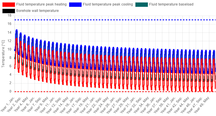
The boreholes have a length of 120 m, use double U DN32 heat exchangers, and are simulated with 25 v/v% MPG and a variable flow rate with a constant temperature difference of 3 °C during both extraction and injection. The heating power is 37 kW with a yearly demand of 67 MWh/year, and for cooling 4 kW and 2.9 MWh/year. This results in a relatively high imbalance, as can be seen in the temperature profile below.
As a first simulation, all boreholes are assumed to be connected directly to the manifold. This results in a highly laminar flow regime (during both heating and cooling), with Reynolds numbers of Re = 875 during extraction and Re = 232 during injection, the difference being caused by a variation in flow rate. The graph for the hydraulic design is shown below.
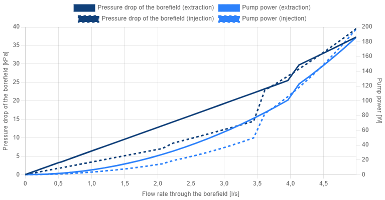
Due to the difference in peak power, the design flow rate for heating is 2.49 l/s, whereas it is 0.35 l/s during cooling. This means that the pressure drop during cooling is almost negligible (≈ 1 kPa) and that the entire hydraulic design is governed by the heating demand. In this case, the total pressure drop is 15.99 kPa, of which 13.21 kPa occurs in the borehole itself and 2.78 kPa in the lateral connections. The estimated pump energy (assuming an efficiency of 70%) is 75 kWh/year.
As a second option, a Tichelmann connection is investigated with groups of 2 boreholes. Therefore, the number of boreholes in Tichelmann is set to 2 in the general tab, resulting in the pressure drop curve shown below.
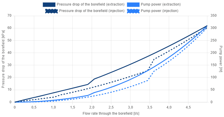
Since a Tichelmann connection ensures that the flow rate through the boreholes remains the same, the pressure drop for the vertical part is identical to that of the direct connection, at 13.21 kPa. The only change occurs in the pressure drop in the horizontal pipes, which is now, due to the doubled flow rate, 10.82 kPa, resulting in an overall pressure drop of 24.03 kPa. The estimated electricity consumption increases to 108 kWh/year.
As a third variation, the boreholes are no longer connected in a Tichelmann configuration, but in series. This changes the flow rate through each borehole (effectively doubling it), which enhances heat transfer. However, since the flow remains laminar (Re = 1776 during extraction), no significant improvement is observed. The minimum average fluid temperature increases from 0.07 °C in the two previous cases to 0.37 °C. The pressure drop graph for this case is shown below.
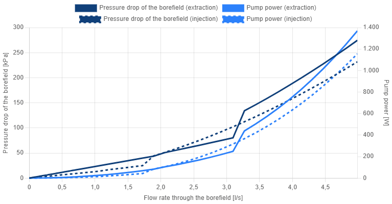
For this series connection, the pressure drop in the borehole increases to 26.04 kPa, since the flow rate is now twice as high as before. The horizontal pressure drop is 10.77 kPa. For the total pressure drop, since the boreholes are connected in series, the pressure drop across the borehole must be counted twice, as the entire flow passes through both. This results in an overall pressure drop of 62.85 kPa, which is significantly higher than in the Tichelmann (or direct) connection. The estimated pump energy consumption is 290 kWh/year.
As a next variation, the double DN32 probe is replaced by a single DN40 probe. In this new situation, the heat transfer becomes turbulent (Re = 2833), resulting in the same minimum temperature of 0.37 °C as in the previous case. However, the pressure drop across a single borehole almost doubles to 41.33 kPa, leading to an overall pressure drop of 93.44 kPa and an estimated pump electricity consumption of 393 kWh/year.
As a final variation, to illustrate the importance of the flow rate assumption, the same simulation is performed with a constant flow rate of 2.49 l/s for the entire borefield (to match the previous situation). The estimated yearly pump energy demand is now 1272 kWh/year, approximately 900 kWh/year higher than in the previous case. The main difference is that, whereas the pressure drop during cooling was previously negligible due to the low flow rate, it now reaches 78.75 kPa.
Conclusion
In this final chapter of Part 4, the hydraulic design was explained for different horizontal connection types (direct, parallel, Tichelmann, and series). Using the concept of hydraulic balancing, it became straightforward to translate the pressure drop of a single borehole into the pressure drop of the entire borefield. It was shown in GHEtool Cloud how the pressure drop can be simulated and what the impact is of moving from a direct connection to a Tichelmann or a series design.
In the next part, we will explore the sensitivities of the design in more detail, both from a thermal and a hydraulic perspective.
Questions
In the hydraulic configuration below, if the inlet flow rate is 1 l/s, what will be the flow rate through each borehole?
Below, an example is given of two boreholes connected in parallel. Can you explain why the two groups above are connected in a Tichelmann configuration instead of a parallel connection?

Why are there two jumps in the pressure drop graph during injection, but only one during extraction in the case of a direct connection to the manifold?
Downloads
- Download GHEtool simulation from this chapter here.