
Geothermal borefields are often used in combination with ground source heat pumps, and the efficiency of the heat pump is required to convert the building load into a ground load. Historically, this efficiency was assumed to be constant, but it is more accurate to use variable efficiencies. In this chapter, this new approach is explained, showing how it can improve your borefield design.
Heat pump efficiency in borefield design
Back in Part 1.5, the heat pump efficiency was introduced to convert the building load into a ground load, which is then used to simulate the long and short term behaviour of the borefield. Typically, the heat pump is modelled using seasonal efficiencies (the SCOP and SEER in the case of cooling), converting both the energy demand and peak power from the building into a ground load. Although this approach is relatively straightforward, there are three main issues with it:
-
By using the SCOP to convert the peak heating power into an extraction peak power, the peak power is overestimated. This is because the peak power efficiency is actually given by the COP rather than the SCOP. Since the COP is typically lower than the SCOP, the ground load at peak moments is overestimated, potentially leading to an oversized borefield.
-
By using an SCOP at B0/W35 to convert the heating demand (and B0/W55 for domestic hot water) into a ground load, it is assumed that the fluid temperature entering the borefield is 0 °C. However, in most designs this only occurs, if at all, after several years, meaning that the average temperature is typically higher. This leads in reality to a higher SCOP, so using a B0/W35 value underestimates the efficiency and therefore the imbalance, which could result in an undersized borefield.
-
As discussed in Part 1.5, the efficiency of a heat pump depends on the fluid temperature of the borefield and will therefore vary depending on the design. However, since the SCOP is historically used as an input rather than an output of a borefield design, it does not change when the design is modified. This is counterintuitive and not representative of reality.
For these reasons, it is clear that the traditional approach has several important shortcomings. In the next section, the influence of the chosen efficiency on borefield design is further illustrated.
Different efficiency assumptions
To quantify the effect of what efficiency is used for the borefield design, three different efficiency assumptions are used:
- The traditional, constant SCOP (at B0/W35)
- A temperature-dependent COP
- A temperature- and part-load-dependent COP
Given these different efficiency assumptions, borefields are designed for three different buildings: a residential apartment building, an office and a multi-utility building, of which some characteristics are given in the table below. In doing so, both the effect on the required borehole depth (i.e. the impact on the actual sizing) and the effect on the final system efficiency are investigated.
| Building | Power | Yearly energy | |||
|---|---|---|---|---|---|
| Heating | Cooling | Heating | Cooling | ||
| Residential building | 66 kW | 97 kW | 153 MWh | 24 MWh | |
| Office building | 214 kW | 371 kW | 118 MWh | 118 MWh | |
| Multi-utility building | 535 kW | 676 kW | 643 MWh | 268 MWh | |
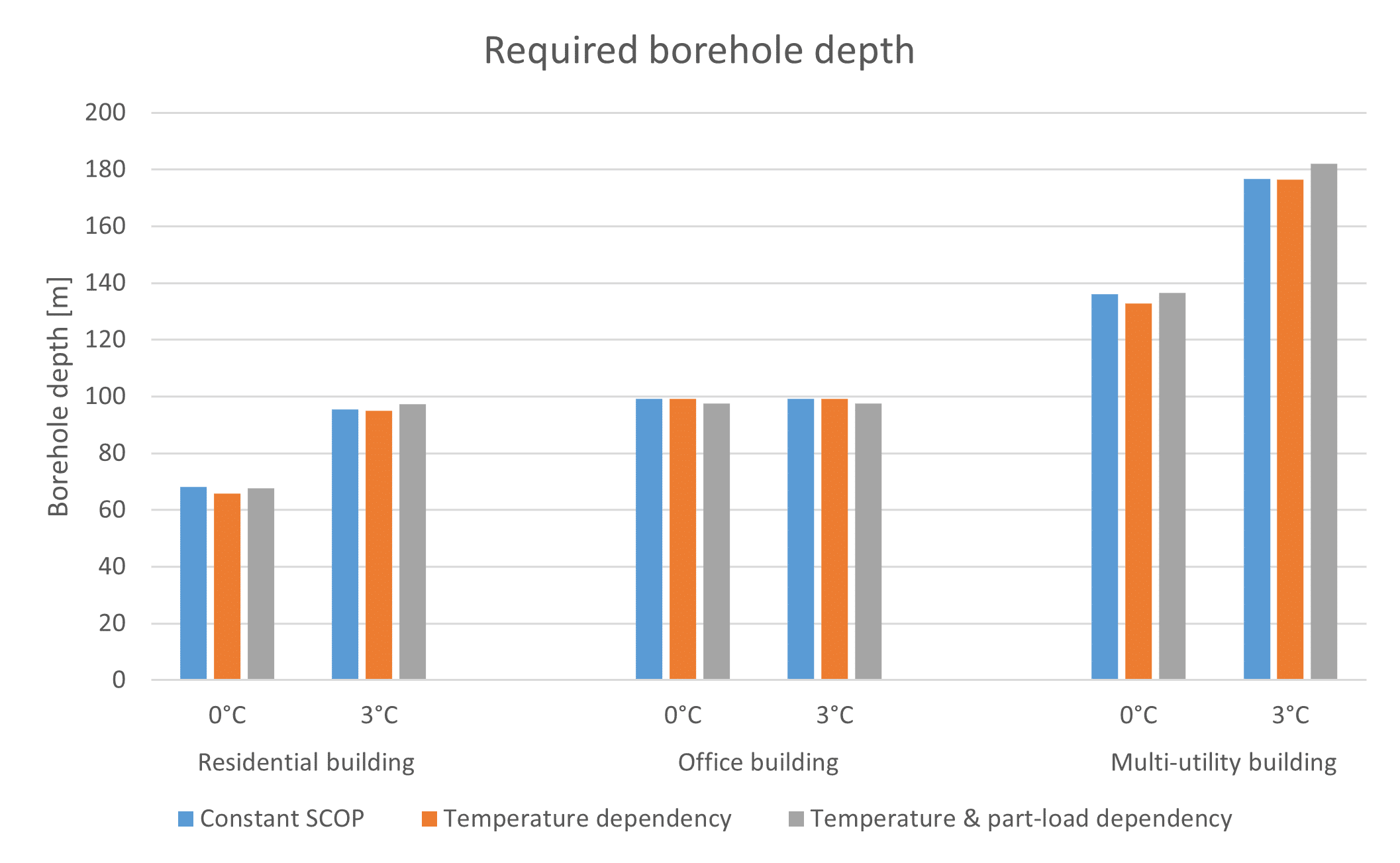
Effect on the required borehole depth
When we look at the effect of the efficiency assumption on the required borehole depth, we see that there is almost no variation between the three different assumptions. In the case of the multi-utility building, there is a slight increase in the required length for a design with a minimum average fluid temperature of 3 °C when including the part-load dependency in the COP. The increase, however, is only 3 percent, which is negligible.
Based on these results, the two errors introduced when working with a constant efficiency versus a temperature- and part-load-dependent one (namely the overestimation of the peak power and the simultaneous underestimation of the imbalance) largely balance each other out.
Effect on the efficiency
Below, the average calculated SCOP is shown for the three different cases. It can be seen that, although there is sometimes a slight difference, the official B0/W35 efficiency is rather close to the temperature-dependent COP. This means that, based on the examples below, there is no real reason to work with only a temperature-dependent COP, since it does not significantly alter either the design or the SCOP.

In contrast, when the part-load dependency is included, there is a significant 10 to 50 percent difference in SCOP between the official B0/W35 value and the expected efficiency. This is due to a double effect:
- The heat pump operates most of the time in the more efficient part-load regime
- In part-load, due to the lower heat extraction, the fluid temperatures are higher, leading to more efficient operation
To further illustrate the importance of part-load dependency, we zoom in on the multi-utility building. Below, the temperature profile is shown.

In the temperature profile above, it is clear that the average fluid temperature fluctuates considerably. Below, a close-up of the COP in the first 5 months is shown for both the temperature-dependent COP and the temperature- and part-load-dependent COP.

COP in the first 5 months for the temperature-dependent COP and the temperature- and part-load-dependent COP of the modulating heat pump. It is clear that the variations are far more pronounced when part-load behaviour is considered than when only temperature dependency is taken into account. Secondly, it can be seen that during peak moments, when both heat pumps operate at full-load, their efficiencies coincide, which is to be expected, since there is no part-load behaviour at these instances.
Since the buildings also have a certain imbalance, the SCOP will change over the course of the simulation period. In the graph below, the SCOP values are shown for each year of the 20-year simulation period for the multi-utility building designed at a minimum temperature of 0 °C.

SCOP variation over time for three different efficiency assumptions.
It is clear that whenever temperature dependency is considered, the efficiency starts higher than it ends, due to the extraction-dominated borefield. Most notably, the pure temperature-dependent COP results in a lower efficiency than the SCOP B0/W35 value after 20 years. This is because this assumption does not include standard part-load behaviour, thereby underestimating the efficiency when operating close to 0 °C.
In contrast, the temperature- and part-load-dependent COP clearly demonstrates the benefit of using a modulating heat pump, where the efficiency is significantly higher than the official B0/W35 value of 4.86 for the SV62 heat pump.
Simulating with modulating heat pumps in GHEtool
Working with temperature- and part-load-dependent efficiency data is not straightforward, as this information is not available in technical datasheets. That is why we collaborate directly with heat pump manufacturers to obtain highly detailed measurement data and create digital twins of their machines. These digital twins are available in GHEtool, so that whenever you are working with an hourly building load, the option appears to select one or multiple modulating heat pumps from our heat pump database.
In the following subsections, different variations of a baseline scenario are simulated using a single heat pump, a cascade configuration of two heat pumps, and a deeper borefield.
Baseline scenario
To illustrate the importance of working with a modulating heat pump, a building with a peak heating demand of 100 kW and an annual heating demand of 200 MWh, and a peak cooling demand of 40 kW with an annual cooling demand of 40 MWh, was used. The hourly load profile is shown in the figure below.

In the baseline scenario, an HP500 heat pump from Enrad, rated at 111 kW, was used, with an official SCOP B0/W35 of 3.41. Using this value, 21 boreholes of 150 m, a double DN32 heat exchanger with 25 v/v% MPG, and a flow rate of 0.3 l/s per borehole, the temperature profile below was obtained.
To illustrate the effect of the different efficiency assumptions, the simulations are carried out with a constant flow rate. However, as discussed in the previous chapter, it would be preferable to design the system using a variable flow rate.

The minimum average fluid temperature is 0.12°C, so just above our threshold of 0°C.
One modulating heat pump
Instead of working with the official SCOP value for the heat pump, let us now select the HP500 heat pump directly from the list and simulate the borefield using it. The new temperature profile is shown below.

It is immediately clear that the temperatures are now lower than in the original design, dropping to −1.02 °C. This is mainly because the average SCOP is 4.66 rather than 3.41, as stated in the datasheet. This represents an increase of 37% in efficiency, increasing the imbalance from 99 MWh per year to 115 MWh per year, which explains the lower temperatures towards the end of the simulation period.
The downward-sloping trend is also visible when looking at the yearly SCOP graph.

With the decreasing temperatures, the heat pump capacity also decreases. In this case, the heat pump is no longer able to fully meet the building demand in the last year, since at −1.02 °C it can only deliver around 94 kW instead of the required 100 kW. In GHEtool, this is shown as a “power shortage” and is illustrated below.

In this case, this is not really a problem, since the missing 6 kW occurs during only one hour of the simulation period.
Two modulating heat pumps
The simulation above was performed with a single HP500 heat pump, rated at 111 kW, which appeared to be sufficient, but perhaps slightly undersized, especially towards the end of the simulation. In this second variation, two smaller HP300 units were selected, each rated at 60 kW, giving a total available power of 120 kW, which is slightly higher than in the previous case. The efficiency curve for this situation is given below.
When working with multiple heat pumps in cascade, a strategy is required to determine when each heat pump will operate. In GHEtool, the approach is that, for every power level, the maximum number of heat pumps is operated in order to keep the average modulation degree, as well as wear, as low as possible, while improving accuracy.
To illustrate this, consider two machines rated at 50 kW and a demand of 30 kW. This could be achieved by operating one machine at 30 kW or by operating both machines at 15 kW. In GHEtool, the second option is always selected. For power demands lower than 30 kW, only one machine is active.

The overall average SCOP is now 4.93, which is 6% higher than in the simulation with a single HP500 unit. However, the temperatures are, again due to the higher efficiency, somewhat lower, now reaching −1.5 °C during peak conditions.
A deeper borefield
As a third variation, we change the borefield design to remain above the 0 °C minimum threshold. Instead of using 21 boreholes of 150 m, the design is changed to 10 boreholes of 250 m, which results in a significantly higher undisturbed ground temperature. In addition, a higher ground temperature also leads to an increase in heat pump efficiency. The temperature profile, as well as the SCOP curve, are shown below. With the same two HP300 units selected, the resulting temperature profile is shown below.

Although the total borehole length decreased from 3129 m to 2490 m (a decrease of 20%), the temperature now remains above 0 °C, with a minimum average fluid temperature of 0.2 °C. The average SCOP, on the other hand, increased from 4.93 to 5.14, truly a win-win situation.

Conclusion
In this chapter, the final major improvement in the accuracy of borefield design was explored: working with variable efficiencies. This not only provides a more accurate design, since both peak powers and the imbalance are more accurately predicted, but also offers additional insight into how the efficiency is influenced by different design choices, such as using two heat pumps in a cascade configuration instead of a single unit, and working with deeper borefields.
Question
In the graph above, all buildings require a greater borehole depth when using 3 °C as the minimum average fluid temperature limit, except for the office building, which has an identical design in both cases. Can you explain why?
Downloads
References
- Peere, W. (2025). Integrating Temperature and Part-Load Dependent COP in Shallow Geothermal Borefield Design. In Proceedings of German Geothermal Congress DGK 2025. Frankfurt (Germany), 18-20 November 2025.
- Peere, W. (2026). Towards a more accurate design of borefields: using variable fluid properties, flow rate and heat pump efficiency. In proceedings of GeoTHERM expo & congress, Offenburg, Germany, 26-27 February 2026. Link