
Traditionally, when designing a borefield, a constant flow rate was used for heating and cooling, during both peak and off peak periods. However, with the introduction of modulating heat pumps, this assumption of a constant flow rate is no longer accurate, and greater insight can be gained by moving towards designs with variable flow rates.
The flow rate
We need a flow rate to transfer energy from the borefield to the building and back, but what flow rate is required? The answer is: it depends on your perspective, since power, temperature and flow rate are all linked through the following relation:$$\dot{Q}=\dot{m}\cdot C_p\cdot \Delta T$$where $\dot{Q}(t)$ is the extraction/injection power in (kW), $\dot{m}$ is the flow rate in (kg/s), $C_p$ the specific heat capacity of the fluid in (kJ/(kgK)) and $\Delta T$ the difference in temperature between the borefield inlet and outlet temperature in (°C).
Since the power varies over time, the equation should be written as a function of time: $$\dot{Q}(t)=\dot{m}(t)\cdot C_p (t)\cdot \Delta T(t)$$where $t$ is the time.
As discussed in the previous part, the fluid properties vary over time, so $C_p (t)$ is determined at each moment by the selected fluid and its temperature at time $t$. Since the power at each hour (or month) is also known, the appropriate combination of flow rate and temperature difference must be found. There are two different approaches: working with a constant flow rate or working with a constant $\Delta T$. Both are explained below.
Constant flow rate
Historically, circulation pumps were single speed, meaning they were either on or off and operated at a constant flow rate. This was not much of an issue, since heat pumps were traditionally also on off. This means that when the heat pump turns on, it demands the maximum power from the borefield and circulates at the maximum designed flow rate. In this situation, there was no real variation in $\dot{Q}(t)$, except for it being either on or off, and therefore $\Delta T$ was also constant.
With the introduction of modulating heat pumps, however, the situation changes. There is now a real variation in power over time, and working with a constant flow rate means that $\Delta T$ becomes smaller when a lower power is required. While such a system may still operate (although some heat pump manufacturers specify a minimum $\Delta T$), it is not the ideal situation. That is why frequency controlled or modulating circulation pumps are now typically used.
Constant $\Delta T$
Instead of predetermining the flow rate, we can also set the temperature difference in the equation above as a constant. This results in a flow rate that varies when the load changes. This is how most heat pumps now control their circulation pump, since each heat pump has an optimal temperature difference at which its efficiency is highest, and the flow is controlled to maintain these ideal operating conditions.
In addition to being more realistic, the flow rate during heating and cooling is typically not the same. For example, if a building has a significantly higher cooling load than heating load, which flow rate should be used as the design value? Setting it too low risks oversizing the system, while setting it too optimistically risks undersizing it. When working with a constant $\Delta T$, a temperature difference setpoint can easily be defined for both heating and cooling.
In addition to this technical reason, there is also a mathematical one. When the flow rate is very low, the corresponding Reynolds number becomes strongly laminar and the effective borehole thermal resistance becomes very high, easily exceeding 10 mK/W (whereas it is normally about two orders of magnitude lower). This could lead to the unrealistic situation where, during periods of very low flow, the temperatures appear to be worse due to this high borehole resistance.
The reason for this is that the effective borehole thermal resistance is, in essence, a steady state approach, which ignores the thermal inertia of the fluid. When the flow rate becomes extremely low, this assumption is no longer valid, and a minimum flow percentage is required to address this. Later in this course, we will return to this steady state modelling of the borehole internals.
Working with a variable flow rate
To illustrate the importance and potential of variable flow rates, let us consider the example of an office building with the hourly temperature profile shown below.
In the profile above, two things are clearly visible:
- The peak power during cooling is almost twice as high as that during heating, and one would therefore expect a significant difference in the resulting flow rate.
- There is considerable variation over the months for both heating and cooling, with significantly lower power during weekends (the white cut outs in the heating profile), meaning that the resulting flow would be far from constant in reality.
To illustrate the difference between working with a constant and a variable flow rate for this building, let us consider a simulation of this office with a borefield of 80 boreholes, a single U DN32 PN16 heat exchanger and a heat transfer fluid of 25 v/v% MPG. A close up of the first year, using both constant and variable flow rates, is shown below.

It is clear that the maximum average fluid temperature is identical in both cases (leading to the same design in the end). This is because the flow rate in the constant case is identical to the maximum flow rate in the variable flow case. However, away from this critical point, the difference in fluid temperatures becomes much more pronounced.
Another observation is that, in the case of a constant flow rate, the fluid temperatures are higher (especially during heating) than in the variable flow rate case. This can be explained by examining the effective borehole thermal resistance below.

In the case of a constant flow rate, the variation in borehole resistance is caused by changes in fluid properties due to their temperature dependency, as discussed in the previous part. However, in the variable flow case, the range in borehole resistance is much more significant, although the two cases do overlap at certain moments halfway through the year (i.e. in summer). This corresponds to the point where the constant flow rate matches the calculated flow rate in the variable case.
At other times of the year, especially during heating when the peak power is much lower, the flow rate is also significantly reduced. As a result, the flow is no longer turbulent and shifts back into a laminar regime with a higher effective borehole thermal resistance. This higher resistance explains why, in the temperature profile above, the temperatures in the constant flow rate case appear more optimistic than those in the variable flow case, but are less accurate.
Potential risks when using constant flow rates
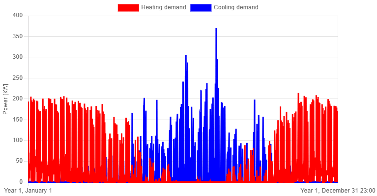
There are also some risks when working with a constant flow rate, especially when dealing with a significant difference between heating and cooling power, or with highly fluctuating peak power in general. To illustrate this, the residential load profile from the previous chapter is shown again below.

When we simulate this project with a constant flow rate of 6.93 l/s for the entire borefield (which corresponds to the peak flow rate during peak injection), using a 25 v/v% MEG heat transfer fluid and a single DN32 PN16 heat exchanger, the result below is obtained.

In the profile above, it is clear that the borefield is sized accurately, staying within the temperature limits, with a minimum temperature after 30 years of 2.64 °C. However, when we select the option to work with a flow rate based on a constant temperature difference (of 3 °C during extraction and injection) instead of a constant flow rate, the result below is obtained.

Since the peak power during heating is lower, the flow rate is no longer 6.93 l/s but only 4.28 l/s. This means that the borefield is no longer turbulent during extraction (Re = 2068 instead of 3496), increasing the effective borehole resistance from 0.1440 mK/W to 0.2401 mK/W. The resulting minimum average fluid temperature is now 1.5 °C, more than 1 °C lower than in the initial simulation. In this case, the borefield is slightly undersized.
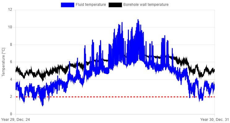
When the same exercise is carried out with the hourly profile, this becomes even more apparent. Therefore, a close up of the last year for the simulation with a constant flow rate is shown below.

When the case above, with a constant flow rate, is compared to the one with a variable flow rate, it is clear that the difference in minimum average fluid temperature (2.09 °C for the constant flow case and 0.93 °C for the variable flow case) is real. It is also clear that, due to the lower flow rate and hence higher borehole resistance, the difference between the fluid temperature and the borehole wall temperature is much more pronounced in the variable flow rate case.
In addition, a clear difference is also visible in summer. With a constant flow rate, the peak temperatures are only reached for a few hours, whereas with a variable flow rate, the maximum fluid temperatures are maintained for a much longer period. This is because, during off peak moments, the flow rate is also lower during cooling, increasing the borehole resistance.
This illustrates another risk when working with a constant flow rate. For example, if a maximum temperature limit is exceeded for only 5 hours, one might be tempted to ignore it. However, when a frequency controlled pump is used, a more accurate simulation with a variable flow rate can lead to very different results, for example 50 hours of exceeding the temperature limit.
Therefore, to avoid undersizing, it is recommended to use a variable flow rate when designing borefields.
Conclusion
Although borefields have traditionally been designed using a constant flow rate (identical for both heating and cooling), this article introduced the feature within GHEtool Cloud to simulate with a variable flow rate based on the assumption of a constant temperature difference between the borefield inlet and outlet.
Working with a variable flow rate has the advantage of saving time and reducing the risk of mistakes. In addition to these practical benefits, variable flow rates provide more accurate results during off peak periods and offer better insight into how the borefield behaves during heating and cooling separately. As shown in one of the examples, this can even lead to a different required borefield size.
In the next chapter, the final major improvement in simulation accuracy is introduced: variable heat pump efficiency.
Questions
In Part 3.2, it was stated that variable fluid properties have an enormous effect on the effective borehole thermal resistance. However, in the figure below, where the borehole resistance is shown for the first year, the resistance for the case of a constant flow rate appears to be more or less constant. How can this be explained in light of the insights from the previous chapter?
Downloads
- Download GHEtool simulation from this chapter here.
References
- Peere, W. (2026) Towards a more accurate design of borefields: using variable fluid properties, flow rate and heat pump efficiency. In proceedings of GeoTHERM expo & congress, Offenburg, Germany, 26-27 February 2026. Link