Supabase, our database hosting service, has a global problem, due to which, GHEtool is not operational at the moment. You can follow the status on https://status.supabase.com/.
You can try GHEtool 14 days for free, no credit card required.
Part 3
Answers
Wouter Peere
Part 3: Answers
In this chapter, we will provide you with the answers to the question at the end of each chapter of the third part or the course.
To get as much out of this design course, we highly suggest you try to solve these questions first for yourself before looking at the solution here.
Please note that, since geothermal borefield design is a rather complicated task, there is sometimes no definitive answer. The solutions we propose here are our interpretation of the questions, but this does not necessarily mean that other solutions would not be valid.
In the case of the residential building, try to find the best combination of peak durations for heating and cooling to achieve a good match with the hourly simulation profile. You can try to do the same for the auditorium building.
The way to do this is to use a trial and error approach to update the peak duration in both heating extraction and cooling injection. In the case of the residential building, the peak duration in cooling should be 4 h, resulting in a maximum fluid temperature of 16.48 °C, which is close to the 16.40 °C obtained from the hourly simulation. During heating, the peak duration should be 110 h to obtain the same average fluid temperature of 2.09 °C.
For the auditorium building, the peak durations should be 3 h and 5 h for heating and cooling respectively, in order to achieve a good agreement between the monthly and hourly simulations.
Since a monthly simulation is a simplification of reality, it is not possible to determine a single peak duration a priori that matches the equivalent hourly simulation. This highlights the importance of using an hourly simulation.
In the last section, the unusual situation of a sudden drop in fluid temperature was shown. Use GHEtool Cloud to explore and find a specific set of design choices that recreates the same effect.
We aim to identify a specific set of conditions under which the fluid transitions from turbulent or transient flow to laminar flow at some point during the simulation period. To determine such a parameter combination, enable the option use variable fluid properties and apply a profile that is extraction-dominated, such as the residential building considered earlier.
In this case, the borefield should be designed such that the flow is just laminar during extraction. Due to the imbalance, the fluid temperature will be lowest in the final year of the simulation and higher in the earlier years. As a result of the higher temperature, the Reynolds number will also be slightly higher, leading to transient flow conditions.
For the residential building, this can be achieved by using a single DN32 PN16 probe and a mixture with 22 v/v% MPG.
Temperature profile of the residential building with the sudden drop.
Please note that, in the profile above, the sudden drop is less pronounced. This is because the magnitude of this drop also depends on the peak power, since the $\Delta T$ between the borehole wall temperature and the fluid temperature depends on both the effective borehole thermal resistance and the peak power. In this case, the peak power is lower, so the effect is less clearly visible.
In Part 3.2, it was stated that variable fluid properties have an enormous effect on the effective borehole thermal resistance. However, in the figure below, where the borehole resistance is shown for the first year, the resistance for the case of a constant flow rate appears to be more or less constant. How can this be explained in light of the insights from the previous chapter?
Effective borehole thermal resistance for one year with both a constant and a variable flow rate.
Using variable fluid properties can result in a significant difference in borehole resistance when a transition between laminar and turbulent flow occurs. In this case, the flow rate is always sufficiently high to maintain turbulent flow, which is why there is little variation. In contrast, in the case of a variable flow rate, the transition between laminar and turbulent flow is clearly visible.
If we look again at the borehole resistance plot above, there appears to be a limit around 0.35 mK/W. Can you explain where this comes from?
This apparent limit is caused by the parameter minimum flow percentage. Since it is assumed, in the graph above, that the minimum flow rate is always 10% of the maximum flow rate, this imposes a lower bound on the flow rate and, consequently, an upper bound on the Reynolds number and the corresponding effective borehole thermal resistance.
Without this limit, the borehole resistance could easily reach 1 mK/W, which is clearly not realistic.
Typically, the efficiency of the heat pump is given at B0/W35, using 0°C as the reference inlet temperature. What would be the corresponding average fluid temperature that we are familiar with when working with GHEtool?
This depends on the flow rate and the temperature difference between the heat pump condenser inlet and outlet. If a temperature difference of 4 °C across the heat pump is assumed, the outlet temperature from the heat pump, that is the inlet temperature to the borefield, is 4 °C lower than the inlet temperature to the heat pump, that is the outlet temperature from the borefield.
This means that when 0 °C leaves the borefield, −4 °C enters, resulting in an average fluid temperature of −2 °C.
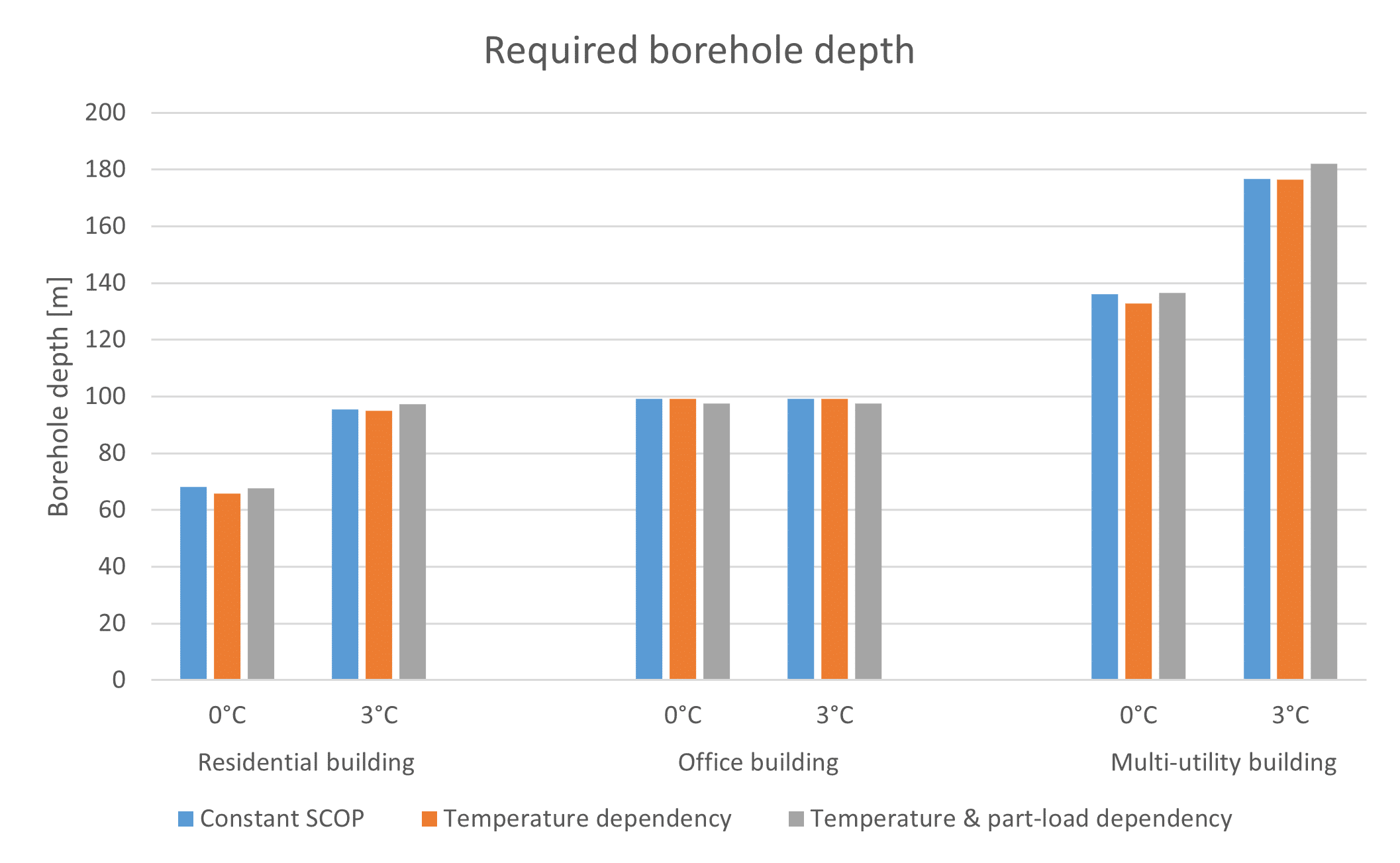
Required borehole depth for three different efficiency assumptions.
In the graph above, all buildings require a greater borehole depth when using 3 °C as the minimum average fluid temperature limit, except for the office building, which has an identical design in both cases. Can you explain why?
If the design does not change when the minimum average fluid temperature limit is varied, this indicates that the system is not constrained by that temperature. In the case of the office building, it is the maximum temperature that determines the required borefield size, regardless of the minimum temperature limit.
Now simulate the last scenario using a variable flow rate, with a temperature difference of 3°C during extraction and injection. How does the design change?
Previously, in the case of a constant flow rate, the flow remained at least turbulent throughout the entire simulation period. When using a variable flow rate, this is no longer the case, and the effective borehole resistance is often higher, leading to lower fluid temperatures and, consequently, lower efficiency.
When transitioning from a constant to a variable flow rate, the overall efficiency of the system decreases from a SCOP of 5.14 to 5.04 due to the higher average borehole resistance and lower fluid temperature. In addition, the minimum and maximum average fluid temperatures change from 0.2 °C and 18.12 °C to −0.1 °C and 18.75 °C.
For injection, this is because the flow rate is lower, leading to a higher borehole resistance of 0.1341 mK/W instead of 0.098 mK/W.
For extraction, the behaviour is more subtle. The two graphs below show the fluid temperature in the 20th year of the simulation period at 08:00 for both constant and variable flow rates.
Simulation of the temperature profile with a constant flow rate.
Although the borehole wall temperature is the same in both graphs, the fluid temperature differs. In the graph with constant flow shown above, the downward trend in fluid temperature can be seen to have shifted to an upward trend a few hours earlier. A similar transition is observed in the case of a variable flow rate. However, at 08:00, there is a sudden jump, which is not present in the constant flow rate case.
Simulation of the temperature profile with a variable flow rate.
This occurs at an hour during which the power is not sufficiently high to reach a turbulent or transient flow regime, and the flow remains laminar in the case of a variable flow rate. As a result, the borehole resistance is higher and the fluid temperatures are lower.
Downloads
Download GHEtool simulation for questions 1.1 and 2.1 here.
Download GHEtool simulation for questions 4.3 here.
You can try GHEtool 14 days for free, no credit card required.
Manage Consent
To provide the best experiences, we use technologies like cookies to store and/or access device information. Consenting to these technologies will allow us to process data such as browsing behavior or unique IDs on this site. Not consenting or withdrawing consent, may adversely affect certain features and functions.
Functional
Always active
The technical storage or access is strictly necessary for the legitimate purpose of enabling the use of a specific service explicitly requested by the subscriber or user, or for the sole purpose of carrying out the transmission of a communication over an electronic communications network.
Preferences
The technical storage or access is necessary for the legitimate purpose of storing preferences that are not requested by the subscriber or user.
Statistics
The technical storage or access that is used exclusively for statistical purposes.The technical storage or access that is used exclusively for anonymous statistical purposes. Without a subpoena, voluntary compliance on the part of your Internet Service Provider, or additional records from a third party, information stored or retrieved for this purpose alone cannot usually be used to identify you.
Marketing
The technical storage or access is required to create user profiles to send advertising, or to track the user on a website or across several websites for similar marketing purposes.