
Historically, the fluid properties (such as density, viscosity, etc.) were often assumed to be constant over the simulation period for your borefield. However, this assumption can lead to significant oversizing of your system, especially when dealing with cooling, as well as give a misleading impression of the long term behaviour of your system.
The importance of fluid properties
Your heat transfer fluid plays a very important role in the thermal behaviour of your borefield. Depending on the flow regime, whether laminar, transitional or turbulent, the heat transfer rate will vary significantly. This has a considerable effect on the effective borehole thermal resistance (as discussed in Part 2.2) and therefore also on the final design of your system.
Temperature-dependent fluid properties
In the graph below, three typical antifreeze solutions are shown: monopropylene glycol (MPG), monoethylene glycol (MEG) and ethanol. Their respective solution concentrations (25%, 22% and 22%) were selected such that the freezing point is identical in all cases, at approximately −11 °C. Pure water is also shown as a reference case.

Both the density (used for the Reynolds number and the flow rate) and the dynamic viscosity (used for the Reynolds number) are very important in the simulation of borefields. It can be seen that the density is more or less constant with temperature, varying by only about ±1% over the temperature range from −5 °C to 25 °C, i.e. the typical operating range of a geothermal borefield. Both MEG and MPG have a significantly higher density than water, whereas a water ethanol mixture has a lower density.
For viscosity, the situation is different. Here, a very significant trend is visible when going from colder to warmer temperatures, with more than a factor of 3 difference in the case of MPG between −5 °C and 25 °C. It is also clear that pure water has a very low viscosity, which is far better than that of the antifreeze solutions.
Temperature-dependent Reynolds number
In the graph below, the Reynolds number was calculated for all fluids using a single DN40 PN16 probe (with an inner radius of 16.3 mm) and a fixed flow rate of 0.2 l/s.

Due to the strong temperature dependency of the viscosity and its relationship with the Reynolds number, the same factor of 3 difference between −5 °C and 25 °C can be observed. It is also clear that the Reynolds number of water, due to its very low viscosity, is always significantly higher than that of any antifreeze solution. This has major consequences for the effective borehole thermal resistance, as will be shown in the next section.
Temperature-dependent borehole resistance
As you may recall from Part 2.2, the fluid regime has a significant impact on the effective borehole thermal resistance. Whenever the Reynolds number is below 2300, the fluid is assumed to be in a laminar state, and above 4000, it is in a fully developed turbulent state. The region 2300 < Re < 4000 is considered to be a transition zone.

In the graph above, a significant drop in the effective borehole thermal resistance is visible when the fluid transitions from the laminar to the transitional regime. The interesting aspect is the temperature at which this occurs. In the colder range (0–5 °C), which is typical when extracting heat from the borefield, the borehole resistance is high due to the laminar flow regime. However, at the same flow rate but at higher temperatures (>12 °C), all fluids become transitional, significantly reducing the borehole resistance.
The interesting point is that, within the same borefield, and given the temperature variation over the seasons, it is entirely possible (as will be shown later) for the fluid to move in and out of the laminar regime depending on the temperature. Assuming constant fluid properties (a typical historical assumption, still used in many other design tools), and therefore a constant Reynolds number and corresponding borehole resistance, is a serious simplification of reality.
Historically, geothermal borefields were used as a stable and relatively high temperature source for ground source heat pumps. In this case, the only temperature of importance is the long term minimum average fluid temperature. Since borefields were always sized to cope with this minimum average fluid temperature, the fluid properties were typically calculated for this worst case condition (or even lower, at the freezing point of the water antifreeze mixture).
More recently, borefields are increasingly being used for cooling, which expands the range of possible fluid temperatures and increases the importance of this temperature dependency. Note that other software, such as Earth Energy Designer or EWS only work with a single fluid temperature and corresponding Reynolds number and borehole resistance. This improvement in accuracy is unique to GHEtool.
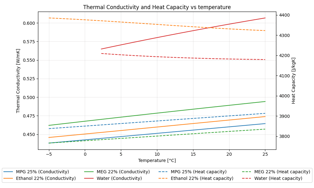
In addition to density and dynamic viscosity, the thermal conductivity of the fluid also plays a role in the borehole resistance. The convective resistance is given by: $$R_{conv}=\frac{1}{hA}$$where $A$ is the heat transfer surface in (m²) and $h$ the convective heat transfer coefficient in (W/m²), which is influenced by the thermal conductivity of the fluid as well as its heat capacity. However, as can be seen in the graph below, similar to density, these parameters do not vary significantly, and the most influential parameter remains the viscosity.
Examples in GHEtool
To illustrate the importance of using variable fluid properties in your design, two different examples will be shown. The first example illustrates their importance for borefield design, whereas the second shows additional insights into borefield behaviour that were previously unnoticed.
Difference in design
Below, a borefield is simulated using constant fluid properties.
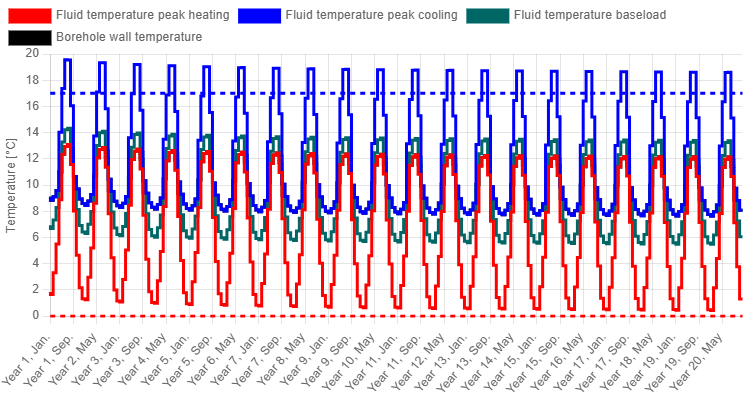
As can be clearly seen, with a maximum average fluid temperature of 19.57 °C, we are significantly above the threshold of 17 °C. If we want to remain below this limit, the borefield size should be increased from 476 m to 654 m (an increase of 37%), resulting in a maximum temperature of 17.3 °C.
However, if we run the same simulation again, now using the assumption of variable fluid properties, we obtain the temperature profile below with a maximum average fluid temperature of 17.5 °C. This is because the Reynolds number during injection is now 4295 (turbulent), resulting in a borehole resistance of 0.1324 mK/W during injection instead of the higher 0.2277 mK/W during extraction.
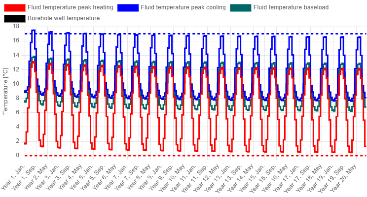
Just by changing the way the fluid properties, and hence the borehole resistance, are calculated, we save nearly 200 m of additional drilling.
Jump in borehole resistance
Since the borehole resistance and the fluid temperature are now bidirectionally dependent on each other, the imbalance becomes apparent again. As a borefield cools down year after year, the viscosity increases, and it can happen that after a certain year, a sudden drop in temperature is observed, as shown in the figure below.

In year 6 of the simulation above, the fluid temperatures are already lower due to the imbalance in the earlier years, and it is no longer possible to achieve turbulent flow from that point onwards. Without the use of variable fluid properties, the temperatures in the first year would also be lower, and this effect (and any possible mitigation) would remain unnoticed.
Conclusion
In this chapter, we discussed the temperature dependency of fluid properties. Since the viscosity of the fluid can change by a factor of 3 over the typical operating temperature range of a borefield, the Reynolds number and effective borehole thermal resistance can also vary significantly.
The traditional assumption of using constant fluid properties in borefield simulations can lead to significant oversizing, particularly when the borefield has a substantial injection load. Another important aspect is that using variable fluid properties can provide additional insights into your design. This was illustrated with an example where, after five years, the temperature dropped below a critical threshold at which turbulent flow could no longer be maintained, causing a sudden decrease in fluid temperature.
Working with variable fluid properties is therefore strongly recommended (and is the default in GHEtool) for more accurate results. The next major improvement in simulation accuracy is the use of variable flow rates.
Question
Downloads
- Download GHEtool simulation from this chapter here.
References
- Peere, W. (2026) Towards a more accurate design of borefields: using variable fluid properties, flow rate and heat pump efficiency. In proceedings of GeoTHERM expo & congress, Offenburg, Germany, 26-27 February 2026. Link