
In February of this year, the heat pump module was released in GHEtool Cloud. This month, the first major update has been released, giving you the option to define your own heat pump as well as specify the emission temperature to the building.
Heat pumps in GHEtool
When you are designing shallow geothermal borefields, it is important to know the actual injection and extraction load in and from the borefield. Historically, this has been obtained by considering the building load on the one hand and assuming a constant seasonal efficiency (or SCOP) for your heat pump to convert it into a ground load. As we pointed out in our article at the end of last year (which you can find here), this leads to three problems:
- Your seasonal efficiency is typically underestimated, since the average fluid temperature is higher than the ‘B0’ one can find in datasheets.
- The peak power on the borefield is overestimated, since the seasonal efficiency is typically higher than the instantaneous efficiency.
- Your efficiency, since it is an input, is independent of your design, which is counter-intuitive to reality.
Due to these three reasons, we released the heat pump module into GHEtool Cloud (read the article here) last February. By collaborating with heat pump manufacturers, we were able to create detailed digital twins of their machines which can be used to simulate the borefield. This not only gives you more accurate results, but also a more realistic image of the real performance of your system.
Although this change has been highly popular, the main feedback we received was a request for an option to define your own heat pumps, which is what we’ll release today.
Efficiency of a heat pump
In order to understand the modelling of the user-defined heat pumps in GHEtool, it is important to understand the theoretical efficiency of the heat pump: the Carnot efficiency. This will be discussed first, after which the simplified heat pump model is explained.
Carnot efficiency
The $T_H-T_L$ part of the equation is also called the ‘temperature lift’, since it is literally the temperature difference between the cold and the warm side of the heat pump, and it plays a central part in the overall efficiency of your machine. The higher this temperature lift, the lower your overall efficiency will be.
Note!
This is exactly the reason why low-temperature emission systems like floor heating are such a good combination with a heat pump. Due to their low temperature requirements (often 35°C or even lower), the temperature lift is rather minimal, leading to very high efficiencies when compared to systems with an emission temperature of 55°C, like, for example, some radiators.
Every heat pump, both ground-source and air-source, modulating or fixed-speed, has this same underlying maximum efficiency, which is why it is used as the backbone of our simplified heat pump model.
Simplified model
The key to the simplified heat pump model is that, for every evaporator-condenser temperature combination, the theoretical maximum efficiency is known from the formula discussed above. However, we need a way to convert this to the real efficiency, which is done with the help of a quadratic correction factor.
Using at least three points (although more will make the fit more accurate), the difference between the theoretical and real efficiency can be quantified, as shown below.
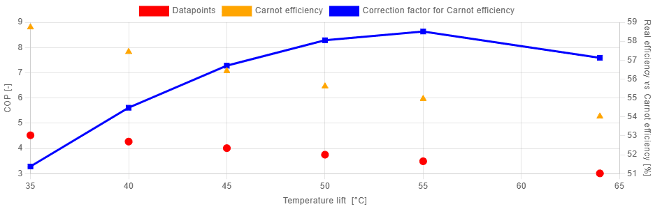
In the figure above, the expected efficiencies are shown as both red dots (for the real efficiency, as given in the datasheet of your heat pump) and orange triangles, which represent the theoretical efficiency. If you divide the former by the latter, you can create a quadratic correlation, quantifying the difference between the theoretical, always-known efficiency and the real efficiency.
Note!
This simplified model only works for fixed-speed, non-modulating heat pumps. In order to model the part-load behaviour accurately, significantly more data points are needed, making the model unfeasible. We are continuing to work on developing a similar, simplified model for modulating heat pumps as well.
Defining your own heat pump in GHEtool Cloud
Inside GHEtool, in the ‘thermal demand’ tab, you have the option to select a heat pump from our database. Previously, these were all predefined, but now there is the option to create your own heat pumps.
Note!
It is only possible to work with a heat pump directly when an hourly load profile is used. When this is not available, an estimated load profile can be created within GHEtool as discussed here.!Note
All the heat pumps you define in GHEtool are also available in your other projects, saving you quite a lot of time redefining machines.
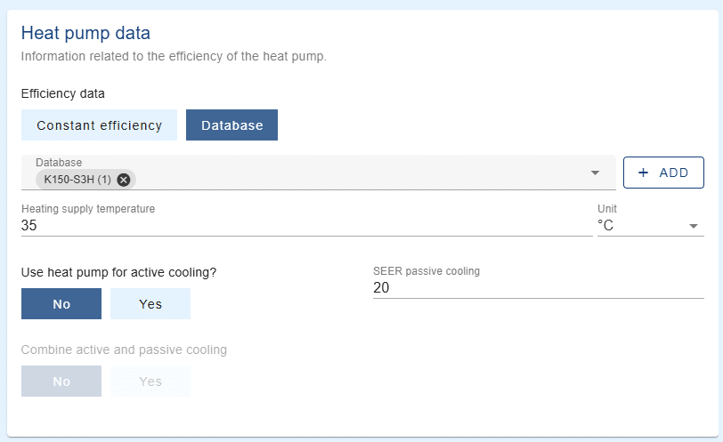
When you add (or edit) a self-defined heat pump, the following information is always required (as shown in the figure below).
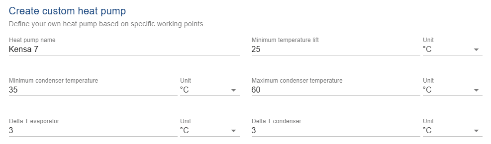
- The name by which your heat pump will be shown in the report and the other projects.
- The minimum temperature lift between the evaporator and condenser, which can vary from heat pump to heat pump.
- The minimum and maximum condenser temperatures, to quantify the working range of your machine.
- The temperature difference between the inlet and outlet of both the evaporator and condenser. This is required since heat pump efficiencies are often defined as Bx/Wy, where x is defined as the evaporator inlet temperature and y as the condenser outlet temperature. In order to work with the average fluid temperatures, the temperature difference should be known.
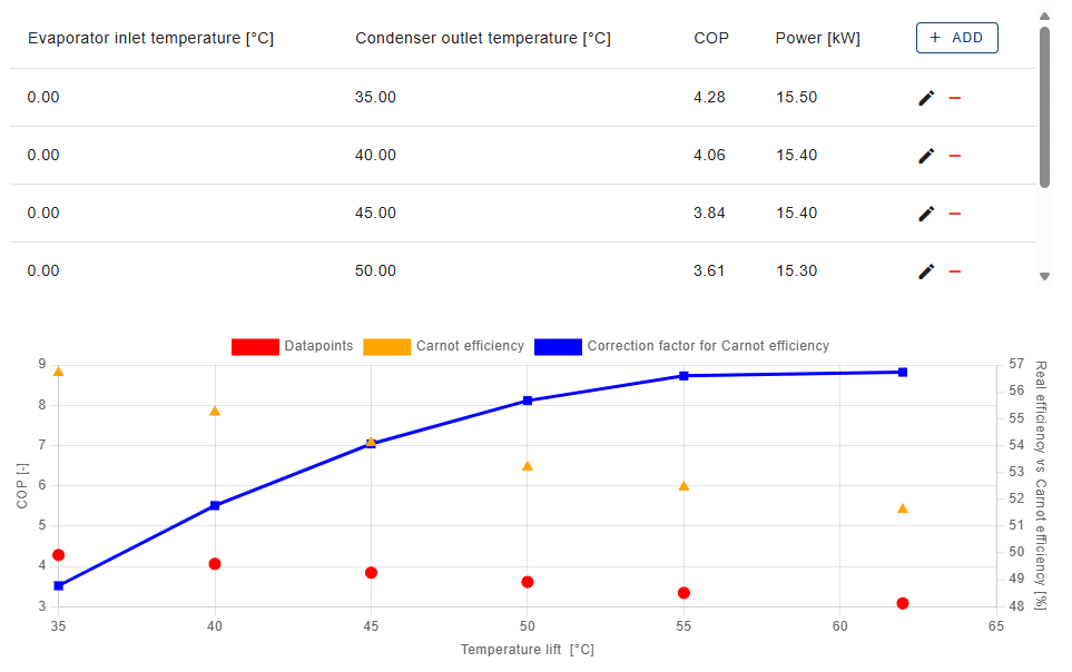
Besides this general information, at least three different, unique working conditions should be provided. For every condition, the evaporator inlet temperature, the condenser outlet temperature, the efficiency, as well as the available power, should be given. Using these points, the correlation can be defined.
!Note
When your heat pump is also used for active cooling, there is no need to enter this data separately, since both the efficiency in heating (COP) and the efficiency in cooling (EER) are thermodynamically linked to each other. That is why defining the heat pump using only the values during heating operation will provide sufficient information to also cover active cooling.
Effect of the emission temperature
In order to show the effect of the emission temperature on the heat pump’s efficiency, let us consider the following simulation with our self-defined heat pump and an emission temperature of 35°C.
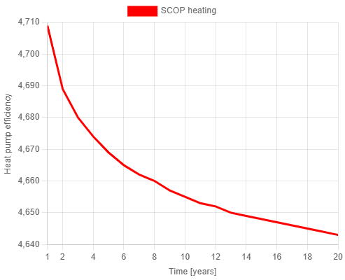
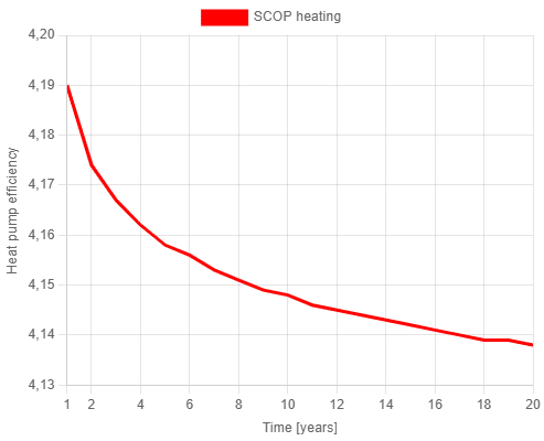
Here, the average SCOP over a simulation period of 20 years is 4.66. When the emission temperature is increased to 45°C, the graph changes and the overall efficiency drops to 4.15. This is simply because, due to the higher temperature lift, the efficiency gets lower, illustrating the importance of having an emission temperature as low as possible.
!Note
When you use your heat pump for active cooling, there is a real chance that you just end up with a straight and constant efficiency, even when there is an extraction-dominated imbalance. This can be caused by the minimum condenser temperature and/or the minimum lift. If you have, for example, a heat pump with a minimum condenser temperature of 25°C and your fluid temperature drops below this 25°C, this will not result in an increase in cooling efficiency, since the heat pump will keep producing 25°C nonetheless.
What is next?
This update marked the first major update to the heat pump module in GHEtool, but it is definitely not the last one. Below are two future updates we are already working on.
- As said, the current simplified model only works with fixed-speed heat pumps. We are researching a similar model that could also model part-load heat pumps, while keeping the same low level of complexity.
- Currently, the emission temperature to the building is constant; however, in reality, this temperature is often a function of the outside temperature: a heating curve. In a future update, this will be implemented, further improving the real efficiency of the ground-source heat pump.
Conclusion
This article described the latest update to the heat pump module in GHEtool Cloud. From now on, it is possible to define your own fixed-speed heat pump and specify the emission temperature for heating, domestic hot water, as well as active cooling.
In the future, this module will be extended further to include a heating curve option, as well as an extension to the current simplified model to cope with modulating heat pumps.
References
- Watch our video explanation over on our YouTube page by clicking here.