
In this article, we introduce the newest feature in GHEtool Cloud: working with variable flow rates. Learn more about this major change, why it is important, the advantages it offers and how it can potentially change the way you design borefields in the future.
A small physics recap
In order to understand the advantages of working with a variable flow rate, we will first recap some of the earlier content in this knowledge base, namely the effective borehole thermal resistance, the Reynolds number and variable fluid properties.
Effective borehole thermal resistance
The effective borehole thermal resistance is one of the most important parameters in geothermal borefield design, as it tells us how easily heat can be transferred from the fluid to the ground. From a design perspective, you always want this resistance to be as small as possible in order to achieve the most efficient design. More information about this resistance can be found in this article.
This resistance is a combination of multiple design criteria, such as the grout, the borehole diameter and the type of heat exchanger used, and is shown in the drawing below.
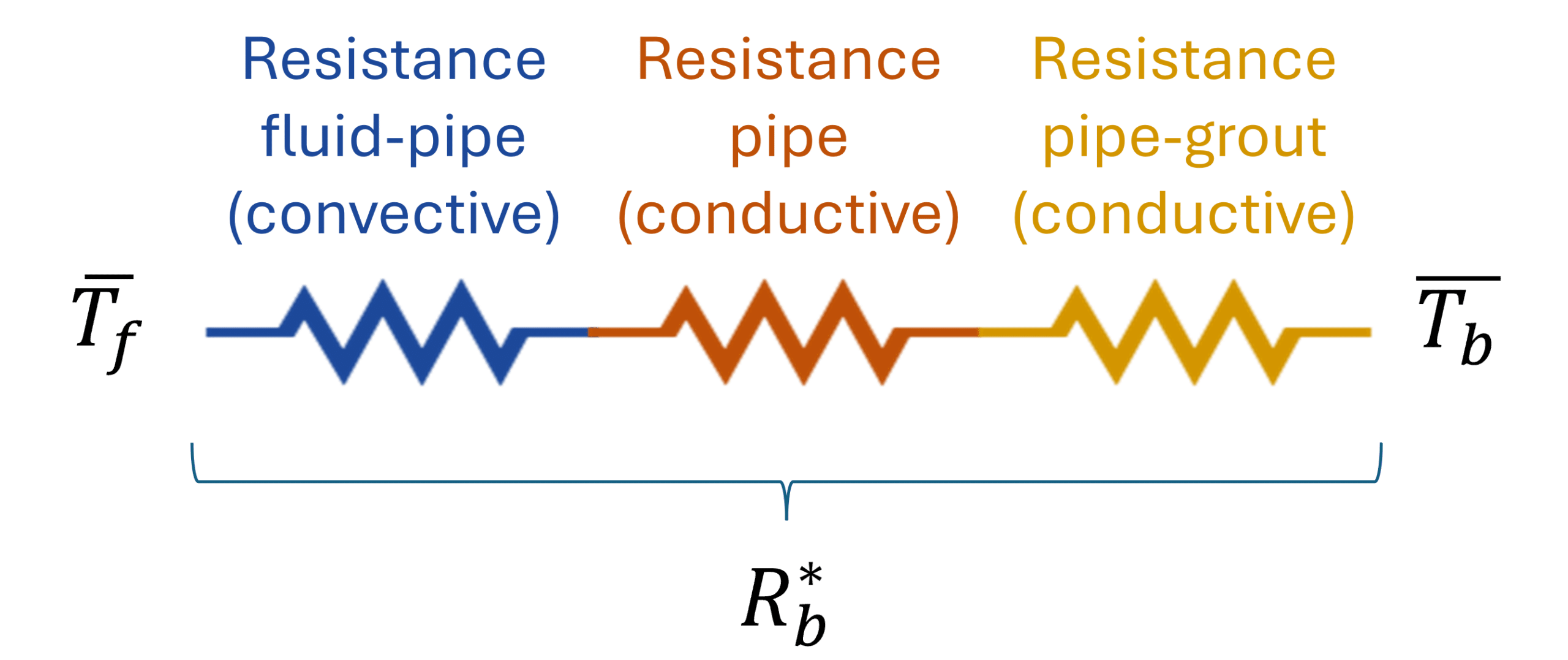
Although all these resistances play an important role in the borehole resistance, there is a major distinction to be made. Both the pipe resistance and the pipe grout resistance are constant and determined during the design phase, since they are conductive in nature. This means that once a certain pipe configuration and grout thermal conductivity are selected, these resistances are constant and will no longer change over the simulation period.
The situation is different for the fluid pipe resistance. Since this resistance is convective, it depends on the fluid properties through the Reynolds number.
Reynolds number
The Reynolds number, which is discussed in more detail in this article is a non dimensional number that provides information about the flow regime of the fluid, whether it is laminar, turbulent or somewhere in the transition zone. This is shown below.

Depending on the flow regime, the convective resistance and therefore also the effective borehole thermal resistance will be different. When the flow is laminar, heat transfer is poorer, although the pressure drop is lower, whereas in turbulent flow the heat transfer is much better.
The Reynolds number is defined as follows: $$Re=\frac{\rho D \dot{V}}{\mu}$$ where:
- $\rho$ is the density of the fluid [kg/m³]
- $D$ is the diameter of the tube [m]
- $\dot{V}$ is the speed of the fluid inside the pipe [m/s]
- $\mu$ the dynamic viscosity of the fluid [pa s]
Besides the diameter of the tube, all the parameters in the equation above vary over the course of the simulation period, causing the Reynolds number, the convective heat transfer and ultimately the effective borehole thermal resistance to change. However, historically, this Reynolds number and the corresponding resistances were assumed to be constant.
This was probably caused by the fact that geothermal borefields were originally sized for use with ground source heat pumps for space heating in buildings, meaning that only the borehole resistance and corresponding Reynolds number at the end of the simulation were considered relevant.
With GHEtool, we aim to increase the accuracy of borefield design, which is why we decided shortly before the summer of 2025 to remove this assumption in two steps:
- Implement variable fluid properties, implemented on 27/05/2025
- Implement variable flow rates, released today
Variable fluid properties
The first step towards a more accurate design was to make the fluid properties, namely density and dynamic viscosity, variable as a function of the fluid temperature. In the graph below, the dependence of the Reynolds number is shown for two monopropylene glycol mixtures at different temperatures.

When you are extracting heat, temperatures are typically around 0 to 5°C, whereas in the mid season or during heat injection they can be 10 to 20°C higher. This temperature difference has a significant effect on the Reynolds number in the simulation, the convective heat transfer, the borehole resistance and ultimately the design.
In our previous example, we showed that this improvement alone can have a significant impact on the design of borefields with a high cooling and heat injection demand. Since the Reynolds number is now calculated more accurately for heat injection as well, peak fluid temperatures are typically lower, leading to more feasible geothermal borefield designs. The full example can be found in our article on this topic.
Variable flow rates
Besides the temperature dependent fluid properties, there is another parameter in the Reynolds number that varies over time, namely the fluid velocity.
Historically, the assumption has been that a constant flow rate is used through the borefield, equal in all months and in both heating and cooling. But is this accurate? Take, for example, a look at the hourly demand profile of an office building.
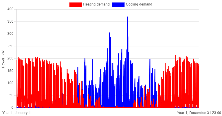
In this profile, you can clearly see that the peak cooling power is almost twice as high as the peak heating power. Is the flow rate really the same in both cases? Imagine heating this building with a modulating heat pump, as discussed in this article). These heat pumps typically also have a modulating flow rate, meaning that even in heating and cooling the flow rate will probably not be the same.
If we want to improve the accuracy of our simulations, it is important to remove the assumption of a constant flow rate, while at the same time ensuring that the simulation remains as fast and easy to use as before. This can be achieved by looking at one of the central equations in heat transfer.
An important equation
One of the key formulas in heat transfer is the following: $$\dot{Q}=\dot{m}\cdot C_p \cdot \Delta T$$ where:
- $\dot{Q}$ is the power injected in or extracted from the borefield [kW]
- $\dot{m}$ is the mass flow rate through the entire borefield [kg/s]
- $C_p$ is the specific heat capacity of the fluid [kJ/(kgK)]
- $\Delta T$ is the temperature difference between the inlet and outlet of the borefield [°C]
In this equation, $\dot{Q}$ is known, since the heating and cooling or extraction and injection demand is an input to the software. In addition, with the implementation of temperature dependent fluid properties, $C_p$ is also known. What remains are the mass flow rate and the temperature difference between the inlet and outlet.
Looking at the formula above, both are interchangeable. Either you set a constant flow rate and the temperature difference will increase or decrease depending on the load, or you set the temperature difference as a constant, which in practice results in a variable flow rate.
It should be clear that the first approach has historically been used, but in reality the second approach is typically more accurate, since in most cases there is a control strategy in place that modulates the flow rate in order to achieve a certain $\Delta T$.
Working with a constant $\Delta T$
If we want to work with a variable flow rate using the constant $\Delta T$-approach, we require some information:
- $\Delta T$ during injection [°C]
- $\Delta T$ during extraction [°C]
- Minimum flow percentage [%]
Since it can occur that the required temperature difference across the borefield is different during extraction and injection, we decided to give you the option to define them separately. In addition, a minimum flow percentage is required, typically between 10 and 30%. This is important, since the circulation pump will generally not operate at 1 to 2% of its peak flow rate.
!Note
When the minimum flow rate is not specified, some unexpected spikes can occur in the simulation when working with an hourly load profile. Typically, due to the way these profiles are constructed, there are some hours with an extremely small heating or cooling demand. In the office example above, the peak power is 350 kW, but there are also values of 1 kW in the simulation. This would result in an extremely low flow rate with an unrealistically high borehole resistance. By defining a minimum flow percentage, this issue is avoided. We return to this later in the article.
Example of working with variable flow rates
To illustrate the importance of variable flow rates, let us return to the office building discussed earlier. We size the borefield and subsequently calculate the borehole resistance and the fluid temperatures using both a constant flow rate and a variable flow rate, while ensuring that the peak flow rates are the same in both cases. The borehole thermal resistance for the first year is shown in the graph below.

It is clear that the borehole resistances obtained using a variable flow rate and a constant flow rate are completely different, although they are identical at certain moments during the summer. This is because the constant flow rate was explicitly set to match the maximum flow rate used in the variable flow case. The second observation is that the variation in borehole resistance for the constant flow rate, which is only caused by varying fluid properties, is smaller than that for a variable flow rate with a constant temperature difference.
The borefield above was designed with a single U probe, which, at the peak flow rate, remained in the turbulent regime throughout the entire simulation period. This explains why the variation in borehole resistance for the constant flow rate is minimal. In contrast, when using a variable flow rate, the peak power during heating and therefore extraction is almost twice as low as the power during cooling or injection. As a result, the flow rate is also significantly lower, leading to laminar flow and a higher borehole resistance, as also discussed in this article.
In the graph below, the consequence of this behaviour for the fluid temperatures in the borehole is shown.

Just as with the borehole resistance, it is clear that the fluid temperatures align during peak cooling in summer. However, when we look at the mid seasons or the periods during heating, we see that the constant flow rate leads to an overestimation of the fluid temperatures. In reality, the borehole resistance will be higher due to a lower flow rate, and therefore the fluid temperatures will be lower.
Advantages
What are the advantages of working with a constant temperature difference assumption instead of a constant flow rate?
- It is more accurate. As shown in the example above, assuming a constant flow rate overestimates the flow rate during periods with a lower peak demand and is therefore less representative of reality.
- It is easier. Previously, you had to calculate the flow rate yourself, either using rules of thumb or the equation mentioned earlier. Now, GHEtool calculates it for you, removing an extra step.
- It provides more insight. With the option to work with temperature differences, you can perform sensitivity analyses by changing the $\Delta T$ during extraction and injection and assess how this affects the design from both a thermal and a hydraulic perspective.
Implemented in GHEtool
This constant temperature difference approach is implemented in the ‘Borehole resistance’ tab in GHEtool. Here, an additional section for the flow rate is available, where you can simply select the constant temperature difference approach instead of the traditional constant flow rate option. It is as easy as that.
!Note
In the examples above, hourly load profiles were used, but a variable flow rate can also be applied in monthly simulations. Therefore, it is available to all users of GHEtool Cloud!

In the result tab, we also updated the hydraulic design section (read more here), as can be seen below.

Further steps
With the current implementation of variable flow rates, the effective borehole thermal resistance is now completely variable over time, providing the most accurate results within this framework. However, the borehole resistance model itself still contains a number of assumptions, since it is based on steady state conditions. This means that the thermal inertia of the fluid and the grout is not taken into account.
For example, when a certain peak power occurs, the effect is immediately visible in both the fluid temperature and the ground temperature. In reality, however, the fluid is heated up first, which can take some time depending on the total volume. After that, the grout responds, and only after several hours does the ground experience this impact. As a result, peak temperatures in reality are typically lower than those predicted by a steady state assumption.
!Note
This is also the reason why thermal response tests take so long. They need to move beyond this transient behaviour, as explained here.
The next step in improving the accuracy of GHEtool Cloud is therefore not to further refine the borehole resistance approach, but to remove it entirely. To be continued.
Conclusion
In this first article of 2026, we focused on variable flow rates. It was shown that the assumption of a constant flow rate is not only inaccurate, but can also give an overly optimistic view during periods when the flow rate differs significantly from the design peak flow rate.
Working with a constant temperature difference between the borehole inlet and outlet is a more accurate way to simulate fluid temperatures without increasing the complexity of the simulation. In fact, since the flow rate no longer needs to be calculated manually, the approach is actually faster.
This marks the completion of our two step process to make the borehole resistance calculation variable over time and more accurate. However, this is not the end of the story, it is only the end of the beginning. In a few months, we will present a new plan outlining how the accuracy of GHEtool can be taken to the next level. Stay tuned.
References
- Watch our video explanation over on our YouTube page by clicking here.