
Typically, when designing borefields, you assume that your project is isolated and that the ground temperature is not influenced by neighbouring systems. In some cases this may be correct, but in others the so called thermal interference between different geothermal systems can be significant. In this article we will discuss the topic of thermal interference and show how GHEtool Cloud can be used to calculate it.
What is thermal interference?
A geothermal system influences the ground temperature. In winter the ground is cooled and in summer it is heated again. In addition to this seasonal effect, whenever there is more heat extraction than injection, a long term temperature drift occurs in which the borefield cools year after year. This effect does not stop at the edge of your property but can easily extend, depending on the ground characteristics, for 50 to 100 m.
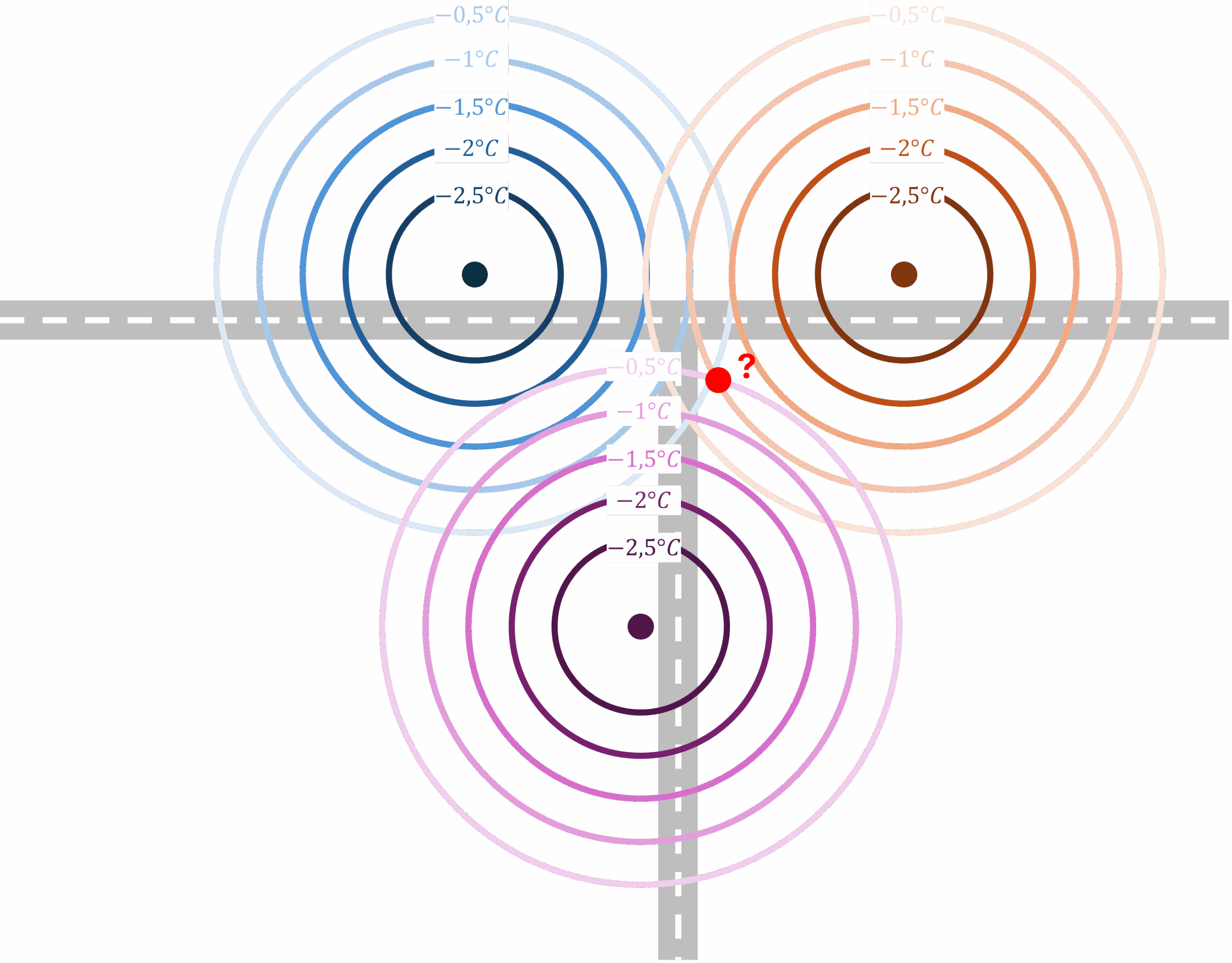
In the illustration above we see a situation where three existing small geothermal systems are located close to one another and the building marked with the red dot wishes to install a ground source heat pump of its own. Typically, the required design information, such as ground, pipe and fluid properties together with the building demand, is entered into GHEtool Cloud and the borefield is designed in such a way that the temperature remains within certain limits (for more information, see our article on the temperature profile).
This approach silently assumes that the geothermal borefield is isolated from the environment and that the surrounding ground is influenced only by itself and not by any other system (more information about the long term behaviour of borefields can be found here). However, in the situation above the three existing borefields have an imbalance that will cool the ground year after year, and the closer you are to these systems the more pronounced this effect will be.
If neighbouring systems are neglected when designing our own, the borefield in the example above will have a minimum average fluid temperature that is two degrees Celsius lower than what was designed, due to thermal interference with the other systems.
!Note
Some regions with a high number of geothermal systems have developed legislation regarding thermal interference. Most notably, the Netherlands has a regulation stating that no interference below -1.5°C is allowed without further justification that the individual systems can still function. They have developed their own ITGBES Excel tool to perform interference calculations when there is a limited number of systems. The thermal interference module in GHEtool Cloud is consistent with Dutch legislation and can be used for interference calculations instead of ITGBES.
Model thermal interference
There are different ways to model thermal interference, but most often the line source solution is used. Since the diameter of the borehole is much smaller than its length, it can be assumed to act as a line. Based on this assumption, two models are typically applied: the infinite line source and the finite line source, both of which are implemented in GHEtool Cloud and are explained below.
Infinite line source
The infinite line source model assumes that the borehole is an infinitely long line. This assumption is reasonable as long as the borehole is relatively long and the neighbouring systems are sufficiently far apart.
The main advantage of this infinite assumption is that the transient three dimensional heat diffusion problem can be reduced to a reasonably simple two dimensional model, since there is no vertical variation along the borehole. This can be illustrated as shown below.

The temperature effect at a distance $r$ from the borehole and at a time $t$ can be expressed as:
$$\Delta T(r,t) = \frac{q}{4\pi \lambda}\cdot E_i \left(\frac{r^2V}{4\lambda t} \right)$$
where:
- $r$ is the distance from the emitting borehole [m]
- $t$ is the time [s]
- $q$ is the average specific heat extraction rate [W/m]
- $E_i$ is the exponential integral function
- $\lambda$ is the ground thermal conductivity [W/(mK)]
- $V$ is the volumetric heat capacity of the ground [J/(m³K)]
Based on the equation above, it is clear that thermal interference is less pronounced at greater distances from the borehole and that the effect increases over time.
Finite line source
The finite line source, as the name suggests, takes into account the actual depth of the borehole and is therefore better suited for accurate calculations of thermal interference when boreholes are close to each other or have significantly different depths.
!Note
The mathematics behind the finite line source is far more complex and is governed by the equation below. For further information, the reader is referred to the scientific literature on the topic, such as Cimmino and Bernier (2014).$$\Delta T_{1\rightarrow2}=\frac{q_1}{2\pi\lambda}\cdot\frac{1}{2H_2}\int\limits_{\frac{1}{\sqrt{\frac{4\lambda}{V}t}}}^\infty e^{-d^{2}_{12} s^2}\left(I_{real}(s)+I_{imag}(s) \right)ds$$
The difference between the two models can be clearly illustrated with the following example. Imagine two boreholes, one 100 m deep and the other 150 m deep, each with a specific heat extraction of 10 W/m. Using the infinite line source assumption, the thermal interference from borehole 1 to borehole 2 is the same as the interference from borehole 2 to borehole 1, since their specific heat extractions are identical.
With the finite line source, the result is different. In this case the interference from the longer borehole to the shorter one is greater than the other way round. This follows from the fact that it requires more energy to influence a borehole of 150 m than it does to influence one of 100 m .
!Caution
Please note that in the models described above, each system is represented by a single borehole. When a system has multiple boreholes, it is represented by one borehole located at the geometric centre of the borefield. This assumption is accurate for up to six boreholes (Groenholland, 2020), after which the distance between the centre and the furthest borehole becomes too large. Whenever a system has more than six boreholes, these can be modelled as different systems with fewer than six boreholes.
Interference and GHEtool Cloud
From today onwards, the interference calculation is available as a new feature within GHEtool Cloud. Below we briefly discuss the inputs and outputs of the method.
Inputs
To perform the thermal interference calculation, some general information is required, such as the ground properties and the simulation period, together with a threshold temperature. This last parameter is not used in the calculation itself, but results below this threshold will be shown in red. Finally, you can select either the infinite or the finite line source model for the interference simulation.

As a next step, the different systems need to be entered. The following information is required:
- The x and y coordinates of the borehole
- The total system length and borehole depth
!Note
For systems with a single borehole this information is identical, but for example with two boreholes of 100 m each, the borehole depth will be 100 m while the total borehole length will be 200 m. - The yearly heating and cooling demand as well as the seasonal performance factor for heating and cooling
!Note
This information is used to calculate the specific heat extraction rate of the borehole, which is the yearly imbalance divided by the borehole depth. This follows the research of Groenholland (2020).
!Hint
When you have many systems, it may be easier to import them as a csv file. For users in the Netherlands, a direct import from the WKOtool is also possible.

Outputs
The result of the calculation is a table showing the interference between each pair of boreholes. The values in red are those that exceed the temperature threshold set in the general input settings. For example, system 1 will experience a total temperature drift of -1.83°C over a period of 20 years due to thermal interference with its neighbours. This table can be exported to a csv file for further analysis.

To further visualise the thermal interference, a heat map is shown. In this map, the darker squares represent systems that have greater thermal interference with one another. The diagonal is white, as a system does not have thermal interference with itself.

Conclusion
This article has discussed thermal interference between different borehole systems and why it is important to consider it when designing a geothermal project. With GHEtool Cloud it is now possible to calculate this thermal interference and quantify the long term temperature drift. The methodology used is fully in line with legislation in the Netherlands and integrates the WKOtool for maximum ease of use.
References
- Watch our video explanation over on our YouTube page by clicking here.