Modelling the FLUX and VARIO probe

As of today, the GEROtherm® FLUX and VARIO probes are available in GHEtool Cloud. In this article, we will shed light on the mathematical model behind these conical probes and explain how it affects their hydraulic and thermal behaviour.

GEROtherm® FLUX and VARIO probes

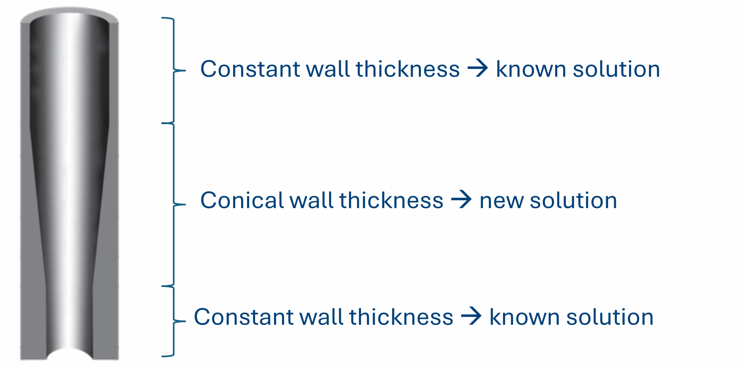
The GEROtherm® FLUX and VARIO probes are two innovative heat exchangers developed by HakaGerodur. They are designed to have the same pressure rating as a regular smooth geothermal probe, but with a lower pressure drop. To achieve this, the wall thickness of the probe is increased towards the end of the borehole, ensuring the required strength where the static pressure is highest. This design gives the VARIO and FLUX probes an overall larger inner diameter, which is beneficial for reducing pressure drop. A vertical cross-section of a FLUX probe is shown below.

!Note
From a modelling perspective, the GEROtherm® VARIO and GEROtherm® FLUX are both considered conical pipes. However, FLUX probes are designed for very deep boreholes (up to 500 m), while VARIO probes are intended for shallower systems (up to 250 m). For more information, you can visit HakaGerodur’s website here.

One pipe, three regions

When we take a closer look at the pipe, we can see it consists of three subsections. The first part of the probe is a regular smooth pipe with a constant wall thickness, for which the solution is already known. The last part of the probe is also a regular pipe with a constant, but different, wall thickness. The region in between, where the wall thickness increases, is where we need to develop a new model.

!Note
Some specific GEROtherm® VARIO probes end after the conical section and do not include a final, ‘regular’ section. This has no impact on the further development of the model.

A first idea might be to simply take an average value of the parameters we are interested in (such as the Reynolds number, friction factor, etc.) between the start and end of the conical section. However, since these parameters are not linear, this does not provide a good estimate. A more accurate approach is to use something called the mean value theorem, which is briefly discussed in the next section.

Mean value theorem

The mean value theorem can be described with the following formula: $$f(c)=\frac{1}{b-a} \int_a^b{f(x)dx}$$

where $a$ and $b$ are the boundary points between which we want to calculate the mean value of the function between points $a$ and $b$ (illustrated by the red squares in the figure above). The idea is to find a green rectangle with the same base width $b−a$ and the same area. The height of this rectangle, $f(c)$, is the average value we are looking for.

!Note
The equation above also allows for analytical solutions. Although a full mathematical derivation is outside the scope of this article, the equation for the Reynolds number in the conical region can be written as: $$\overline{Re}(x)=\frac{-1}{x}\frac{4\rho \dot{V}}{\pi \mu}\frac{1}{2a}\left[ln(D_{in,start}-2ax)-ln(D_{in,start})\right]$$ where $x$ is the position in the conical part of the probe [m] and $a$ is the rate of increase in wall thickness, $\dot{V}$ the volume flow rate [m³/s], $D_{in,start}$ the initial wall thickness at the start of the conical part [m] and the other parameters $\rho$ and $\mu$ are respectively the fluid density [kg/m³] and the dynamic viscosity [Pa.s]. For more information on the Reynolds number, the reader is referred to this article.

Behavior of the conical probes

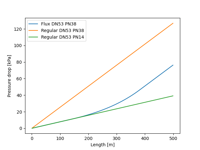
Pressure drop of a double GEROtherm® FLUX DN53 PN38 probe in function of depth for a 25% MEG mixture @3°C and 0.9 l/s.

Initially, the pressure drop of the FLUX probe follows the same trend as that of the regular PN14 probe, with the deviation starting at 140 m—where the conical section begins. Beyond this point, the pressure drop increases until it becomes more or less parallel to that of the regular PN38 probe. It is clear that for a system 500 m deep, this difference in wall thickness has a significant impact on the overall pressure drop and, consequently, on pump energy consumption.

In the graph below, the depth is kept constant at 500 m, while the flow rate is varied. Initially, the pressure drops are very similar due to the laminar flow regime. Around 0.4 l/s, the regular PN38 probe begins to transition into the turbulent zone, which is visible as a sudden increase in pressure drop.

The same transition occurs at a higher flow rate for the PN14 probe. This is because its larger inner diameter results in a lower flow velocity, delaying the onset of turbulence. For the FLUX probe, the transition also begins around 0.4 l/s, but it is less pronounced—since only part of the probe has the same PN38 wall thickness—resulting in an overall lower pressure drop across all flow rates.

For a probe of this length, the figure looks slightly different from the one we saw in our previous article, where the drop between the laminar and turbulent regimes was more pronounced. Here, since the probe is relatively long, this effect—although still present—is smaller. As you can see, the thermal performance of the conical FLUX probe is comparable to that of the other probes up to 0.5 l/s, but it starts to deviate beyond that point. Interestingly, the thermal performance is better than that of the regular PN38 pipe, due to its overall thinner wall thickness.

!Note
Due to its conical design, the heat transfer rate is not uniform along the depth of the probe, as turbulence and pipe resistance vary. However, since the g-functions are calculated using a boundary condition of uniform borehole wall temperature, this variation does not affect the accuracy of the model. More information on the g-function calculation can be found here.

GEROtherm® FLUX and VARIO probes in GHEtool Cloud

All the GEROtherm® FLUX and VARIO probes from HakaGerodur are now available in GHEtool Cloud in the drop-down list of all the heat exchangers.

Conclusion

This article described the mathematical model for the GEROtherm® FLUX and VARIO probes developed by HakaGerodur. It was shown that using a simple average to model the conical section is not sufficiently accurate, and that the mean value theorem provides a more reliable approach.

The results demonstrated that, especially at greater depths, the pressure drop is significantly reduced thanks to the conical design and its overall larger inner diameter. The thermal performance was similar to that of regular probes at lower flow rates, but at higher flow rates, a clear thermal improvement was observed compared to a regular pipe of the same pressure class.

References

• • Watch our video explanation over on our YouTube page by clicking here.