Long-term effects: g-functions

In the last chapter, we talked about the short-term temperature effects and the borehole resistance. In this chapter, we’ll introduce the concept of g-functions and how they can be used to explain the seasonal and yearly variation in the borehole wall temperature.

Thermal behaviour of borefields

In the last chapter, a distinction was made between short-term temperature effects and long-term temperature effects in the borefield. The short-term was basically a power problem, where the effective borehole thermal resistance expressed the relationship between the borehole wall temperature and the fluid temperature. The higher the (peak) power onto the borefield, the larger this difference became, being linearly proportional to the borehole resistance.

Today, the focus will be on the energy management of the borefield and its seasonal and yearly effects on the temperature. To understand that, we need to talk about the concept of g-functions.

G-functions

The physics behind a borefield is quite complex, as it involves a three-dimensional transient heat diffusion problem. Now, without going to deep into the mathematical details, we immediately feel that thermal interaction of the borehole with the ground does not stop at the borehole wall, but it continues in the ground. This means that:

1. There is an interaction between the different boreholes in the same borefield.
2. There is an interaction between the borefield and the surrounding ‘infinite’ ground, since heat transfer does not stop at the edge of the project site.
3. There is an interaction between neighbouring systems.

To model these effects, Eskilson developed the concept of a g-function in his PhD thesis in 1987: a dimensionless function that describes how the borehole wall temperature evolves when a constant load is applied. Each borefield design (with its unique configuration, depth, geological conditions etc.) has its own characteristic g-function, which can be seen as the thermal fingerprint of the system’s long-term behaviour. An example is shown below.

In the graph above, a constant heat injection of 1 kW was applied to a certain borefield. You can see that the temperature increases but, over time, the rate of increase becomes smaller. This can be understood as follows: in the beginning, when heat is injected into a borehole, it affects only its immediate surroundings. Since this ‘region of influence’ is initially quite small, the temperature increase is relatively high. Over time, more of the heat is dissipated further into the ground, and the region of influence expands. The borehole now has more volume through which it can dissipate heat, so the temperature increase becomes smaller.

This ever-increasing (or decreasing, in the case of heat extraction) but less-than-linear trend describes the long-term behaviour of the borefield, where the imbalance causes the ground to heat up or cool down over the years at a decreasing rate. Understanding how your design influences this characteristic g-function will help you manage your imbalance and long-term behaviour more effectively.

There are three different (analytical) ways to calculate the g-functions of a certain field, depending on how the boreholes are modelled. These are:

1. The infinite line source (ILS)
2. The finite line source (FLS)
3. The in(finite) cylindrical source (ICS/FCS)

The infinite line source is the easiest to work with, because do to the assumed infinite borehole depth, the problem of the thermal interaction between different boreholes, becomes two dimensional. It is typically accurate when boreholes are rather deep and far apart and can for example be used to calculate the interference between neighbouring systems.

The finite line source assumes, as the name suggests, that the borehole is a line of finite length. This is the most common model for borefield simulations, since it is rather accurate for boreholes of shallower depth and densely packed.

The cylindrical source takes into account the real geometry of the borehole, by working explicitly with a volumetric element instead of an infinite thin line. This is important when considering the transient dynamic effects within the borehole at short timescales, which will be discussed later in this course.

The figure below shows the g-function using the different models on a semi-logarithmic scale.

Here, the different assumptions become very clear. On the short timescale, the infinite cylindrical heat source deviates from the ILS/FLS solution due to the real geometry in the model. At longer timescales, the difference between the ILS and FLS models becomes clear. The higher the ratio between the borehole length and the radius (i.e. how good the borehole approximates a line), the longer it takes for the FLS to deviate from the ILS solution.

To calculate the finite line source, the concept of spatial superposition is used. This implies that the resulting thermal effect on one borehole (or borehole segment) is equal to the weighted sum of all contributions. This is shown in the figure below.

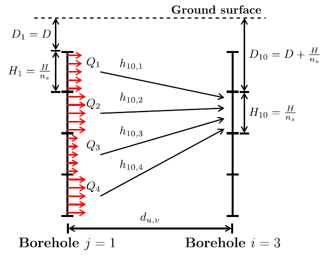
As can be seen, every borehole is divided into segments (in this case 4) and every segment has a specific heat exchange with the ground, indicated by $Q_i$. Depending on your boundary condition (constant heat flux, constant borehole wall temperature (used in GHEtool Cloud) or mixed inlet fluid temperature), the $Q_i$ can be different for each segment.

To calculate the g-function of the entire borefield, the thermal interference between all segments is calculated. In the image above, the thermal effect of all four segments (weighted by their respective power and distance) onto one segment of another borehole is calculated. This is repeated for all segments of all boreholes, until everything gets weighted to end up with one general thermal response of the entire borefield.

For a more detailed mathematical explanation, the reader is referred to the literature at the bottom of the chapter.

Determining parameters

There are three important parameters that influence the g-functions and where we as a borefield designer have influence on: ground thermal conductivity, borehole spacing, and borefield configuration. Below, each of them is discussed in more detail.

Ground thermal conductivity

When we discussed the ground properties in Part 1.3, we introduced the ground thermal conductivity as the ability of the ground to conduct heat. If the ground has a higher thermal conductivity, your borefield can dissipate its heat faster, and it can more rapidly utilise a larger region around the borehole to exchange heat. This lowers the g-function and therefore reduces the impact of the imbalance on your long-term behaviour.

Although you cannot change the ground thermal conductivity directly (as it is a geological given for a certain project location), you can determine the drilling depth. Imagine for example that there is a bad conducting ground layer at 80 m deep. Drilling into that layer, will lower the overall thermal conductivity of your ground, impacting the g-functions and the long-term effect.

Borehole spacing

As mentioned earlier, one of the effects captured in the g-function is the thermal interaction between the different boreholes in the borefield. The further apart your boreholes are, the less they will influence each other and the more energy can be exchanged with the surrounding ground. This effect is shown in the figure below.

When the boreholes are spaced further apart (for example, 10 m), the g-function is clearly lower. This is because the greater spacing between the boreholes allows heat to be transferred more easily to the surrounding ground, reducing the g-function and therefore the impact of ground imbalance on the design.

You can also observe that for all the different borehole spacings, the g-functions converge at shorter timescales. This is because, initially, the boreholes only interact with the immediate environment and they do not yet ‘feel’ each other. After a certain time, these regions of influence grow and start to overlap and the curves diverge due to the thermal interaction between the boreholes. This divergence happens first with the 6 m spacing, as the boreholes interact with each other sooner than those separated by 8 or 10 metres.

Borefield configuration

A final parameter that influences the g-functions is the configuration of the borefield. If the boreholes are placed close together in a rectangular (or dense) grid, the boreholes in the centre have a harder time transferring heat to the surrounding ground. This results in a faster increase in the borehole wall temperature, which is reflected by a steeper g-function. However, if the boreholes are arranged in a single line, they can more easily exchange heat with the surrounding ground. This leads to a lower g-function and, therefore, a reduced impact of imbalance on the final design.

Groundwater flow

The g-functions described above consider only conductive heat transfer in the ground. This assumption allows for fast ground response calculations but neglects a factor that can significantly influence some projects: groundwater flow.

When groundwater flows through the borefield, it carries heat or cold downstream via a process known as advective heat transfer, resulting in a temperature plume, as illustrated in the figure below.

This advective heat transfer can play a major role in the long-term thermal evolution of the borefield. Since groundwater transports part of the imbalance away from the field, the borehole wall temperature tends to remain much more stable over time. This can allow for a smaller borefield size, especially in systems with high imbalance. However, in the case of seasonal thermal energy storage (STES), this effect can be disadvantageous, as some of the stored energy may be carried away by the groundwater, reducing the system’s storing capacity and overall efficiency.

If the groundwater flow is known and your borefield suffers from long-term imbalance, it’s best to orient the longest dimension of the borefield perpendicular to the groundwater flow. This orientation maximises the positive influence of advective heat transfer, by minimising the contact between your borefield and the flow. Conversely, placing the borefield parallel to the groundwater flow increases the risk of losing heat to the environment.

Accounting for groundwater flow is challenging. It is a parameter that is both difficult to estimate and highly influential in simulation results. If you want to model these effects specifically, you can use dedicated software such as Modflow, Feflow or seequent. However, in general practice, assuming only conductive heat transfer will likely result in a conservative estimate, as groundwater flow often improves performance in reality.

From g-function to long-term effect

Until now, we have talked about the g-functions in terms of a constant injection or extraction of heat into or from the ground. However, in reality, the geothermal load varies over time. To account for this, we can use a method called temporal superposition to transition the g-functions for a constant load to a varying one. This is done in three steps, illustrated in the image below.

1. Load decomposition
   First, the real geothermal load (on a monthly or even hourly timescale) is broken down into a series of constant loads. For example, if we have a load of 1, 0.5, -0.5, and 0 as shown in the graph on the left, we can decompose this into constant loads of 1, -0.5, -1, and 0.5, as shown in the middle graph, each starting at different times.

   What we do is the following: we begin with a constant load of 1 starting at t=0. At t=20, the original load drops from 1 to 0.5 (a change of -0.5), so we add a constant load of -0.5 starting at t=20. If we sum the original 1 and the new -0.5 from t>20, we end up with 0.5, as intended. This continues: at t=40, the load drops to -0.5 (a change of -1), so we add a constant load of -1 starting at t=40. The result, $=-0.5$, matches the original data. This process continues for every step in the load profile.

2. Applying the g-function to each constant load
   Now that the load is decomposed into different constant components, we can apply the g-function to each one individually. This is shown in the transition from the middle figure to the one on the right. Each time a new constant load starts, a corresponding g-function is initiated. For example, at t=0, we apply a g-function multiplied by the load of 1. At t=20, we apply a new g-function multiplied by -0.5, and so on. All the g-functions are the same, since they only depend on the borefield design, but they are scaled according to the magnitude of the load.

3. Summing the g-functions
   Finally, to determine the resulting ground temperature over time, we sum all the active g-functions vertically. From t=0 to t=20, only one g-function is contributing. From t=20 to t=40, we sum two g-functions, and from t=40 to t=60, three, and so on. The final result is the black line in the graph, which describes the borehole wall temperature over time.

By using this method of temporal superposition, both the seasonal variation in the ground and the long-term thermal behaviour can be calculated using constant and elegant g-functions.

Conclusion

In this chapter, the long-term effect of the borefield was explained with the concept of g-functions that model both the interaction between the different boreholes in the borefield as well as the interaction of the borefield with its surroundings. Having a smaller g-function was beneficial for the long-term effect and hence for cases with significant imbalance.

This ground response could be influenced by placing the boreholes as far apart as possible, opening up the configuration as much as possible and trying to install the borehole into good conducting ground layers.

In the next chapter, the knowledge of the short- and the long-term behaviour of the borefield will be used for our first geothermal borefield simulation.

Question

References

• • Eskilson, P. 1987. Thermal Analysis of Heat Extraction Boreholes. PhD thesis, University of Lund.
  • Cimmino, M., Bernier, M. 2014. A semi-analytical method to generate g-functions for geothermal bore fields, International Journal of Heat and Mass Transfer, Volume 70, Pages 641-650, ISSN 0017-9310, https://doi.org/10.1016/j.ijheatmasstransfer.2013.11.037
  • Picard, D. 2017. Modeling, optimal control and HVAC design of large buildings using ground source heat pumps systems. PhD thesis, Catholic university of Leuven.
  • Molina-Giraldo, N., Blum, P., Zhu, K., Bayer, P., & Fang, Z. (2011). A moving finite line source model to simulate borehole heat exchangers with groundwater advection. International Journal of Thermal Sciences, 50(12), 2506-2513.
  • Gao, Z., Hu, Z., Chen, T., Xu, X.,  Feng, J.,  Zhang, Y., Su, Q.,  Ji, D. (2022). Numerical study on heat transfer efficiency for borehole heat exchangers in Linqu County, Shandong Province, China, Energy Reports, Volume 8, Pages 5570-5579, ISSN 2352-4847, https://doi.org/10.1016/j.egyr.2022.04.012.
  • Loveridge, F. (2012). The thermal performance of foundation piles used as heat exchangers in ground energy systems. PhD thesis, University of Southampton, UK.