
As of today, the MuoviELLIPSE from Muovitech is available in GHEtool Cloud. In this article, we shed light on the mathematical model behind this elliptical probe, covering both the fluid dynamics and the internal heat transfer within the borehole.
MuoviELLIPSE
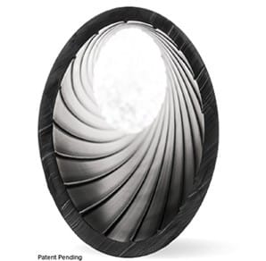
The MuoviELLIPSE is, as the name suggests, an elliptical heat exchanger developed by Muovitech. Like its counterpart, the TurboCollector, the MuoviELLIPSE features multiple small fins along its inner surface. These fins are oriented alternately in clockwise and counterclockwise directions along the length of the pipe. Acting as passive turbulators, they are designed to induce turbulent flow behaviour at lower flow rates, thereby enhancing heat transfer.
In standard smooth pipes, the transition to turbulence typically begins at a Reynolds number of around 2300. However, due to the internal geometry and elliptical shape of the MuoviELLIPSE, turbulence is initiated at approximately Re = 1850.
Model development
As is clearly visible, the MuoviELLIPSE differs from traditional smooth round pipes in two ways:
- The fluid behaviour inside the probe is affected by the internal fins and the elliptical shape.
- The heat transfer outside the probe, but within the borehole, is influenced by its irregular geometry.
To model the MuoviELLIPSE correctly, both aspects must be considered. The first aspect is addressed using Computational Fluid Dynamics (CFD), and more specifically Direct Numerical Simulation (DNS), and is discussed first. The heat transfer within the borehole is then calculated using the Boundary Element Method (BEM).
Computational Fluid Dynamics
Computational Fluid Dynamics (CFD) is one of the most important fields in engineering today. It is used to simulate fluid behaviour in chemical plants, optimise the shape of aircraft wings to maximise lift, assess the aerodynamic performance of vehicles, predict wind turbine output, and much more. When it comes to modelling the thermohydraulic behaviour of the MuoviELLIPSE, CFD is the preferred method.

!Note
The thermohydraulic simulation of the MuoviELLIPSE follows a similar methodology to that used for the development of the TurboCollector model. For more information on the methodology employed, the reader is referred to this article. As with the TurboCollector, the fluid dynamics results were generated by Niklas Hidman (2026), whose article is referenced below.
Within the field of CFD, there are various approaches to modelling turbulence, ranging from simplified and computationally efficient methods such as Reynolds Averaged Navier Stokes (RANS) and Large Eddy Simulation (LES) to the highly computationally demanding Direct Numerical Simulation (DNS). Using DNS, fluid behaviour is resolved down to the smallest spatial and temporal scales, allowing even the finest turbulent structures to be captured.
Since the fins that induce turbulence are themselves relatively small, only DNS is capable of accurately capturing the true thermohydraulic behaviour of the MuoviELLIPSE.
Below, the result of such a DNS simulation for a pipe with internal fins is shown (Hidman et al., 2026).
!Note
Although the results shown below are taken from Hidman et al. (2026) and relate to the TurboCollector, the same principles also apply to the MuoviELLIPSE.

In the image above, the first CFD simulation was performed for a Reynolds number of 3300, corresponding to fully turbulent flow. By systematically reducing the Reynolds number in the simulation, the flow gradually transitions out of the turbulent regime and enters a transitional regime characterised by local flow disturbances, as illustrated by the case with Re = 1800. For Reynolds numbers below 1700, the flow regime becomes fully laminar.
For the MuoviELLIPSE, the transition from laminar to transitional flow occurs at approximately Re = 1850, compared to the traditional value of around Re = 2300 for a smooth pipe. This behaviour can be observed in the two correlation graphs shown below.

The graph on the left shows the friction factor (more information can be found here) as a function of the Reynolds number for both a smooth elliptical probe, which serves as a reference, and the MuoviELLIPSE. It is clear that, at a Reynolds number of approximately 1850, the probe with internal fins begins to deviate from the smooth pipe behaviour and moves towards the friction factor associated with turbulent flow. Once the flow becomes turbulent, it follows the familiar decreasing trend with increasing Reynolds number.
The same behaviour can be observed when examining the Nusselt number, which is a measure of convective heat transfer. At the transition threshold of approximately Re = 1850, the Nusselt number increases sharply, indicating a significant enhancement in heat transfer. As a result, the effective borehole thermal resistance decreases, as will become clear later in this article.
!Note
Note that, for the Nusselt number, multiple simulations were performed for different Prandtl numbers, indicated by the various colours. A detailed explanation of the Prandtl number is beyond the scope of this article, but for geothermal applications it typically ranges from approximately 20 (green) to 75 (red), depending on the fluid properties, such as the type of antifreeze used, and the fluid temperature.The results show that the observed increase in heat transfer at the transition to turbulent flow occurs across the entire range of relevant Prandtl numbers.
Boundary element method
The second challenge in modelling this pipe is accounting for its elliptical shape. For traditional smooth circular pipes, the internal heat transfer equations can be solved analytically. However, this is no longer possible for non-circular geometries.
To overcome this limitation, a numerical approach in the form of the Boundary Element Method (BEM) was employed.
!Note
The application of the Boundary Element Method to shallow geothermal borefields was inspired by and co-developed with Prof. Massimo Cimmino.
The Boundary Element Method (BEM) is a numerical technique used to solve linear partial differential equations (PDEs), such as those governing heat transfer. In the present case, it transforms the original two-dimensional problem into an equivalent one-dimensional problem defined along the boundaries of the pipes and the borehole wall.
Put simply, rather than solving for the entire temperature field within the borehole, it is sufficient to solve an equivalent heat transfer problem along the pipe surfaces and the borehole wall. This concept is illustrated graphically below.
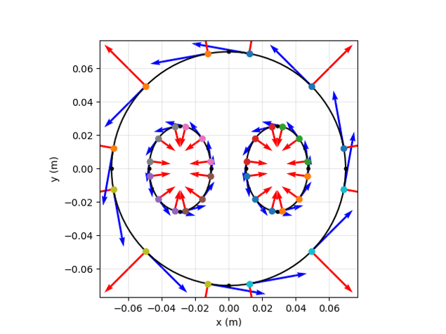
In the figure, the different points represent the nodes at which the heat transfer equations are solved. The arrows indicate the tangential and normal components of the heat transfer. By discretising the pipe geometry in this way, it becomes possible to accurately account for the true elliptical shape of the probe.
The main drawback of the BEM is that it is computationally intensive and therefore too slow for direct use within GHEtool. To make the model sufficiently fast for practical simulations, an Artificial Neural Network (ANN) is trained using the results of the high-fidelity BEM simulations. This approach combines the best of both worlds: an accurate, geometrically representative model for calculating heat transfer within the borehole and an ANN that enables these calculations to be performed efficiently within GHEtool.
!Note
Artificial Neural Networks (ANNs) are already used within GHEtool to accelerate the calculation of g-functions, which form the basis of the methodology used to determine the required size and depth of a borefield. For more information the reader is referred to this article on the topic.
Based on the models discussed above, the effective borehole thermal resistance and pressure drop of the MuoviELLIPSE are examined below.
Simulation results
Using the friction factor and Nusselt number correlations derived from the CFD simulations, together with the Boundary Element Method (BEM), the effective borehole thermal resistance and pressure drop characteristics of the MuoviELLIPSE can be evaluated. The results are discussed below.
Effective borehole thermal resistance
The graph below shows the effective borehole thermal resistance for both the MuoviELLIPSE DN45 (PN16) and a smooth DN45 circular probe used as a reference. The results were obtained for a borehole diameter of 120 mm and a fluid consisting of 25 vol.% monoethylene glycol (MEG) in water for both probes. A borehole depth of 100 m was assumed, together with a grout thermal conductivity of 1.5 W/(mK).

The sudden decrease in effective borehole thermal resistance, marking the transition from laminar to transitional flow, occurs at a lower flow rate for the MuoviELLIPSE than for the smooth reference probe. This behaviour is a direct consequence of the internal fins, which promote turbulence at lower Reynolds numbers and thereby enhance heat transfer.
Another notable observation is that, under fully developed turbulent flow conditions, the effective borehole thermal resistance of the MuoviELLIPSE and the smooth reference probe converges, with the circular probe exhibiting a slightly lower thermal resistance. As shown in the cross-sectional view below, the circular pipes are positioned slightly closer to the borehole wall than the elliptical ones. Once the fluid flow becomes turbulent, the contribution of the grout resistance to the overall borehole thermal resistance becomes increasingly significant. In this regime, locating the pipes closer to the borehole wall is advantageous, as it reduces the heat transfer path through the grout.

The advantage of an elliptically shaped probe is that it can be installed more easily in boreholes with smaller diameters. As can be seen from the cross-sectional views above, the MuoviELLIPSE has more clearance within the borehole, providing additional space for installation and positioning. As a result, it can potentially be installed in a smaller borehole than an equivalent circular probe.
A comparison between a circular DN45 probe installed in a 120 mm borehole and a MuoviELLIPSE installed in a 90 mm borehole is presented below.

In the graph above, the transition to turbulent flow still occurs at approximately the same Reynolds number. However, the MuoviELLIPSE now outperforms the smooth circular probe across the entire range of flow rates. This improvement is primarily due to the smaller borehole diameter, which reduces the grout resistance and therefore lowers the overall borehole thermal resistance.
Pressure drop
In the graph below, the pressure drop is shown for both the MuoviELLIPSE DN45 and the smooth circular DN45 reference probe.

One can see that the pressure drop starts to increase sooner for the MuoviELLIPSE than for the circular pipe. This is because, just as with the TurboCollector, the enhanced turbulence at lower flow rates comes at the cost of an increased pressure drop. In addition, a clear difference in pressure drop between the elliptical and circular pipes is visible.
This is because the hydraulic diameter of the two probes is not identical. The circular DN45 PN16 probe has an internal diameter of 36.8 mm, whereas the hydraulic diameter of the elliptical probe is 34 mm. This smaller diameter results in a slightly higher flow velocity for a given flow rate and hence a higher pressure drop.
!Note
The hydraulic diameter is a concept used to model non-circular geometries by defining an hydraulic diameter that would give them the same hydraulic properties as a circular pipe. This hydraulic diameter is defined as:$$D_h=\frac{4A}{P}$$where $D_h$ is the hydraulic diameter in (m), $A$ is the cross-sectional area in (m²), and $P$ is the wetted perimeter in (m). Since the ratio $A/P$ is slightly smaller for an elliptical probe than for a circular one, the hydraulic diameter is also slightly smaller.
MuoviELLIPSE in GHEtool
From today onwards, the different MuoviELLIPSE probes, ranging from DN32 to DN63 and available in both PN10 and PN16 variants, are available in GHEtool Cloud under the ‘Borehole Resistance’ tab. Try them out today!

Conclusion
This article discussed in detail the mathematical modelling of the MuoviELLIPSE, based on the recent work of Hidman N. (2026) for the heat transfer inside the probe, as well as the Boundary Element Method to account for the elliptical shape.
It was shown that the clockwise and counterclockwise rotating fin design creates a transitional flow regime starting at around Re = 1850, whereas the transition to turbulent flow in a smooth pipe starts only at around Re = 2300. Due to its elliptical shape, this probe can be installed in a smaller borehole diameter, thereby improving the effective borehole thermal resistance.
The friction factor is higher for the MuoviELLIPSE in the range 1850 < Re < 2300 due to the induced turbulence, but it converges towards the smooth pipe solution in both the laminar and fully turbulent regimes. However, due to the smaller hydraulic diameter associated with the elliptical shape, the overall pressure drop remains higher than that of its circular counterpart.