Calculate required borefield size and depth

The design of shallow geothermal borefields is always a little bit trial and error, but what if it is not? In this chapter, we’ll introduce the automated method that allows you to calculate the required borefield depth and size simultaneously.

Borefield design (traditional approach)

Designing borefields, especially bigger systems, is always a little bit of trial and error, especially if you are working with irregular configurations. To make life a little bit easier, methods to calculate the required borefield depth (like the one discussed in Part 7.2) exist.

However, as we discussed in the last chapter, these methods sometimes do not yield any solution, especially when the borefield is limited by the maximum fluid temperature limit. The main solution to this gradient error was to increase the number of boreholes in the system until the algorithm converged, which can be quite time-consuming for bigger systems. This is where the method to calculate both the required borefield size and depth comes into view.

In order to understand how this algorithm works, it is important to understand the nature of the problem and how Bayesian optimisation can be used to solve it.

Bayesian optimisation

When searching for the optimal borefield size, configuration and depth, there are a number of parameters that can be varied. These include the shape of the configuration such as U-shaped, L-shaped, box-shaped, rectangular shaped or dense shaped, the number of boreholes in the length and width direction, the spacing in the length and width direction as well as the borehole depth.

In the optimisation world, each of these parameters that requires tuning is called a hyperparameter, and there are different strategies for solving this type of problem, as shown below.

A first possible solution is to perform a traditional grid search. In this approach, you define the ranges you want to explore, for example the number of boreholes in the length direction being [1, 2, 3, 4, 5], and you combine all possible values. Next, you calculate the required borehole depth for each combination, and the best result becomes your final answer. This approach is of course very time-consuming, especially for bigger systems, where easily more than 2000 combinations should be checked.

Another, less structured approach is to use a random grid. Here, the search options do not form a grid structure since the input parameters are selected randomly. After a number of searches and trials, the best solution found is presented. This method is also rather time-consuming and offers low certainty that a good solution will be identified, due to the random nature.

The last option, which is the method implemented in GHEtool Cloud, is to use Bayesian optimisation. The idea is that we start with some random combinations of input parameters for the borefield design and calculate the required borehole depth for each configuration. Based on those initial simulations, the algorithm constructs an uncertainty function that indicates where it is most likely to find the best solution, and it then iterates statistically towards it. This process is also illustrated in the figure below.

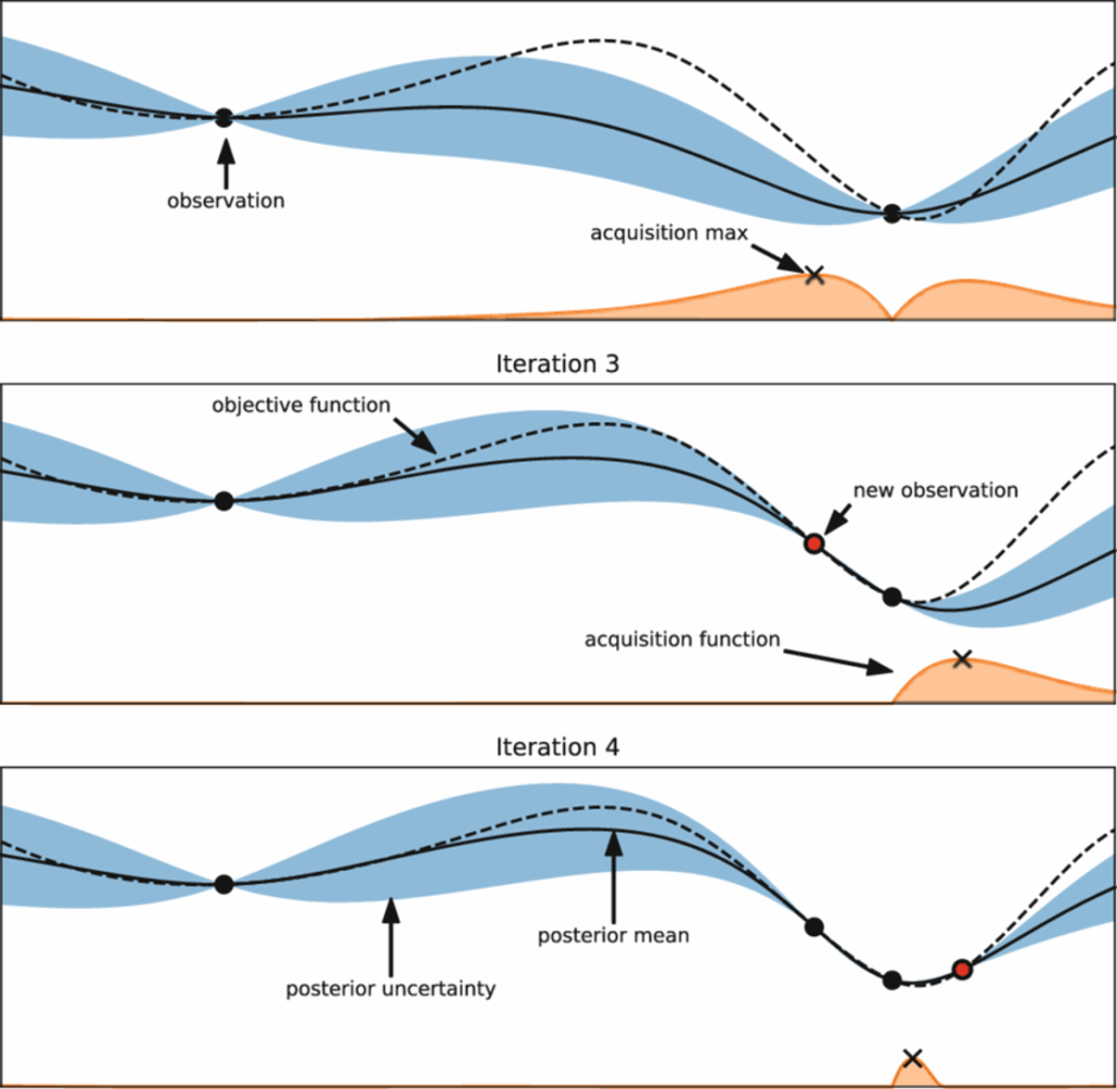
The picture above shows different iterations of the optimisation algorithm. In the top image, two calculations have already been performed, so at these two points we know exactly what the value is, in our case the total borehole length and/or the total number of boreholes. The further you move away from these simulations, the greater the uncertainty becomes.

In the next iteration, number 3, we want to try another borefield configuration with the highest chance of giving us an even lower total borehole length. Therefore, we search for the lowest point within our uncertainty bounds shown in blue and calculate a new point. By repeating this process, the uncertainty bounds become smaller and we converge towards an optimum.

Calculate required size and depth in GHEtool Cloud

If you want to use this method in GHEtool Cloud, you simply have to selected the aim: ‘calculate required size and depth’ in the ‘General’ tab. Afterwards, the ‘Borefield’ tab will be changed from a configuration selector to a place where you can enter both the borefield inputs as well as some optimisation settings. Both will be discussed below.

Borefield input bounds

In the print screen below, the borefield input bounds are giving.

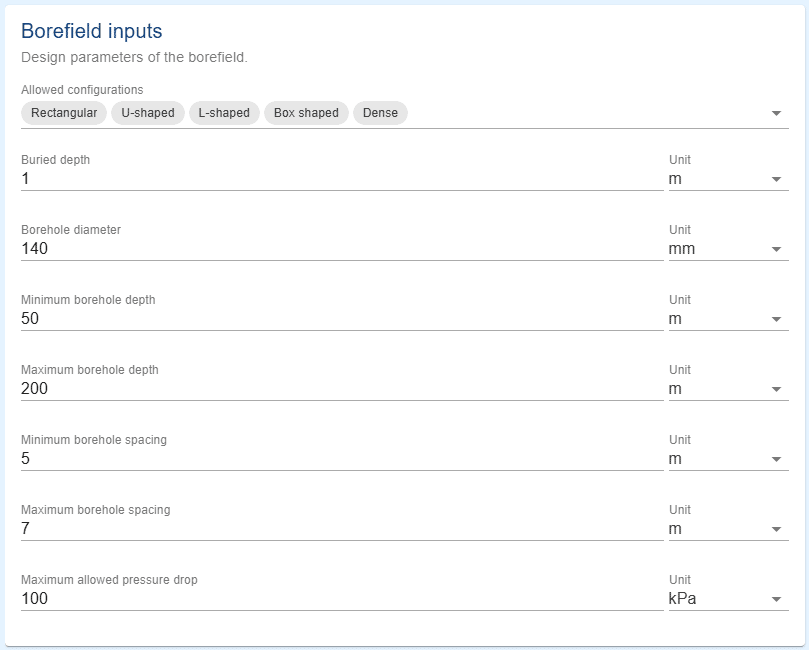
As said, the calculate required borefield size and depth method searches only regular configurations of which you can set the boundaries here. (The buried depth and the borehole diameter are given as constants and are not part of the actual optimisation.)

The parameters that you can tweak are:

• The minimum and maximum allowed borehole depth. Whereas the method from the previous chapter could not consider any maximum drilling depth for legal and/or geological reasons, this methodology can.
• The minimum and maximum allowed borehole-to-borehole spacing.
• The maximum allowed pressure drop per borehole, in order to make sure that the installed circulation pump can handle the pressure drop of the optimised system.

Optimisation settings

Below the optimisation settings are shown.

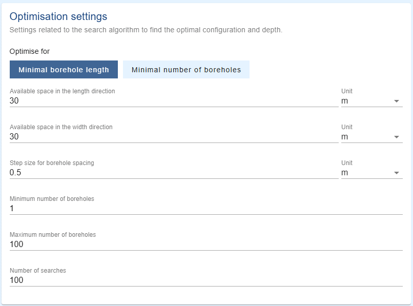
When it comes down to the optimisation settings, one can either optimise for the minimal borehole length or the minimum number of boreholes, since depending on your project, either one can be wanted. The available space in length and width direction determine the maximum number of boreholes in each direction together with the step size for spacing.

The minimum and maximum number of boreholes are no strict requirement, but they can help to speed-up the algorithm. If you for example have a very small project, it makes no sense to let the Bayesian algorithm search for fields with 100 boreholes and reducing the search space in this way can make the algorithm faster.

Lastly, the number of searches determines the number of iterations the Bayesian search will do. The larger this number, the higher the chance that you have found the optimal case. Typically, 50-100 is already enough to achieve this goal.

Example

In order to show the power of this method, let us revisit the example from Part 7.2, where a project with a demand of 22 MWh/year with a peak power of 15 kW in heating and a demand of 7.6 MWh/year with a peak power of 10 kW was considered. The case has a double U tube, 25 v/v% of MPG and a variable flow rate with a constant temperature difference of 3°C.

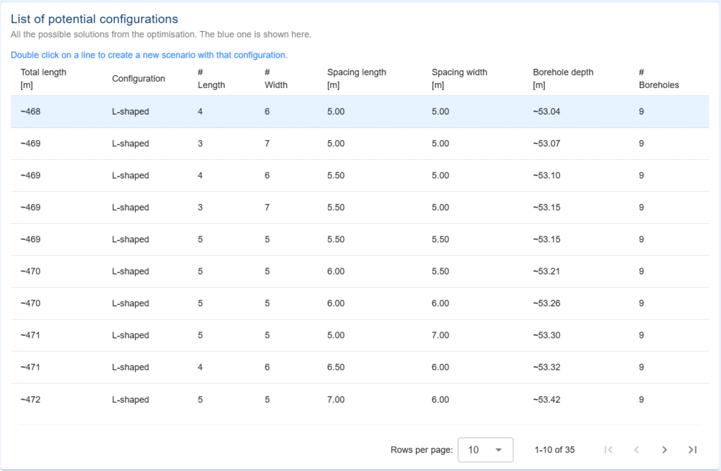
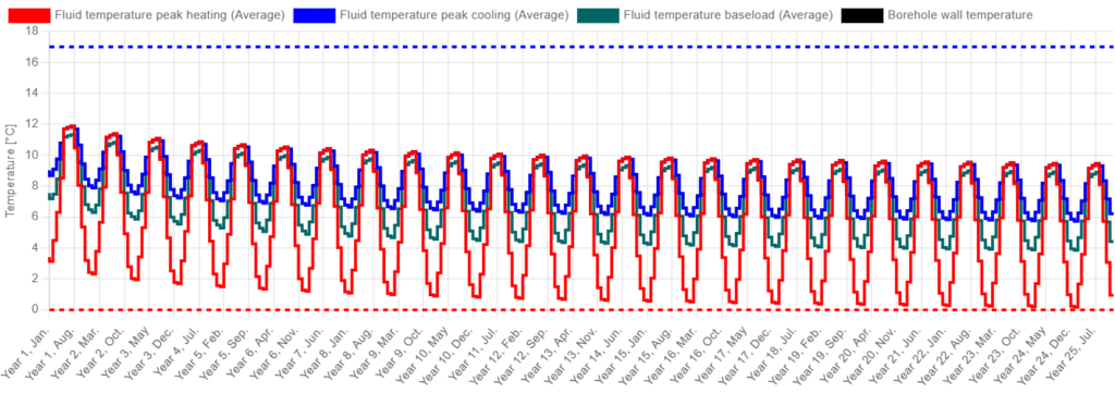
Calculating the required size and depth with the minimum total borehole length yields a borefield with 9 boreholes of 53.04 m deep for a total of 468 m. The temperature profile is given below.

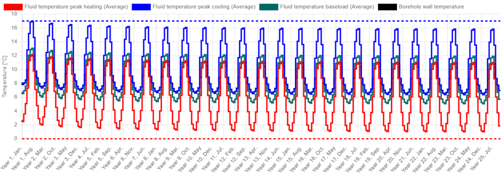
In the temperature profile above, it is clear that this borefield (as was also clear in the last chapter) is limited by the maximum fluid temperature. That is why, the gradient error in mind, a rather shallow borefield was obtained. In fact, looking at the table of all found solutions, the first 10 all have rather shallow drilling depths.

In contrast, running the same optimisation now with the optimisation for minimum number of boreholes yields a result with 5 boreholes of 116 m for a total borehole length of 575 m (more than 100 m than in the previous case). This clearly illustrates the importance of selecting the right optimisation goal, since the result can be significantly different.

As another example, a case with 8 MWh/year of domestic hot water, 25 kW in heating with 45 MWh/year of energy demand and without any cooling is considered. Since the borefield is now clearly extraction dominated, let us increase the maximum borehole depth to 300 m but limit the acceptable pressure drop to 50 kPa. The result with the minimum total borehole length is shown below and has 4 boreholes of 175 m deep, for a total of 696 m. The temperature profile is given below.

In the profile above, it is clear that the minimum limit is now the design criterium for the borefield. Notice also that the result for the minimum total borehole length and the minimum number of boreholes is, more or less, identical.

When the maximum acceptable pressure drop is increased to 150 kPa, the solution changes. Now, 3 boreholes with a depth of 199 m (for a total of 595 m) is the ideal solution. This option was not visible before, since the pressure drop is slightly above 100 kPa.

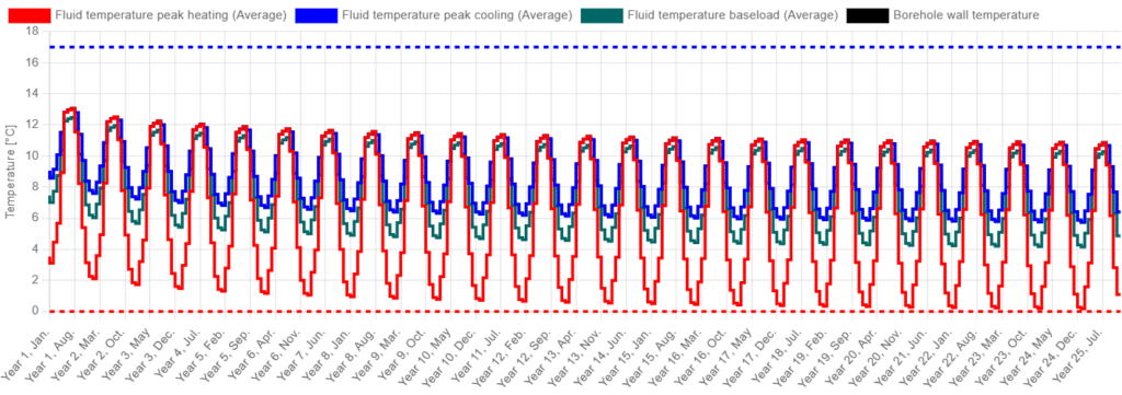
To further improve the design, let us switch to a double DN40 instead of DN32 to lower the pressure drop. When this is done, the required borefield size is reduced to 2 boreholes of 251 m borehole depth with a total borehole length of 499 m. The temperature profile of this is shown below.

Conclusion

The calculate required size and depth method allows for a fully automated borefield sizing experience. With the help of Bayesian optimisation, the algorithm searches for the ideal configuration and corresponding borefield depth, overcoming the gradient error. In two examples in GHEtool, the power of this method was illustrated.

References

• Olson, R.S., Moore, J.H. (2019). TPOT: A Tree-Based Pipeline Optimization Tool for Automating Machine Learning. In: Hutter, F., Kotthoff, L., Vanschoren, J. (eds) Automated Machine Learning. The Springer Series on Challenges in Machine Learning. Springer, Cham. https://doi.org/10.1007/978-3-030-05318-5_8

Questions

Downloads

• Download GHEtool simulation from this chapter here.