
Knowing the ground properties (as well as the borehole resistance) is a prerequisite of good borefield design and the best way to measure them in situ is with a thermal response test, or TRT in short. In this chapter, this measurement is explained, together with how it can be analysed in GHEtool Cloud.a
What is a Thermal Response Test (TRT)?
When it comes to the design of borefields, there are a few very important parameters: the ground thermal conductivity and undisturbed ground temperature (see Part 1.3) as well as the effective borehole thermal resistance (see Part 2.2). Although all three can be estimated or, in the case of the ground properties, looked up in tables, there is always a difference between theory and practice. For large projects, or when no accurate data is available, it is recommended to measure these parameters in situ. This can be done with a Thermal Response Test.
A TRT is always performed on a sample borehole that is representative of the way the borefield will be constructed later. This means it has the same drilling diameter, depth, grouting, heat exchanger, etc.. Once this borehole is installed, it is left for a few days to allow the grout to harden and the borehole can return to thermal equilibrium with the environment after being disturbed by the drilling.
After that, a TRT rig is brought to the site and connected to the borehole. This rig includes a data logger to measure both inlet and outlet fluid temperatures, a circulation pump, and an electric heater. An illustration of the test site is shown in the figure below.

After installation, the circulation pump first runs for couple of hours without the heater being turned on. This mixes the fluid and gives a reading of the initial undisturbed ground temperature over the whole borehole length. After this initial period, the heater is turned on at a constant power and the fluid temperature starts to increase.
After 48 to 72 hours, or sometimes even longer, enough temperature measurement data has been acquired to also determine the ground thermal conductivity and the effective borehole thermal resistance. The most common way of doing this is with the help of the infinite line source method.
Although a constant-power TRT is by far the most common, it is not the only way of performing a thermal response test. In recent years, some alternative approaches have been suggested.
- Constant-temperature TRTs inject heat at a constant temperature in the ground instead of having a constant power. This simplifies the analysis since no estimate of the volumetric heat capacity of the ground is needed (Aydin et al., 2019).
- Flow-controlled TRT allows the users to have both a constant heat injection as well as having a constant inlet and outlet temperature. This removes any inconsistancies between a constant heat flux and constant inlet temperature TRT, offering higher accuracy (Aydin et al., 2024).
- Constant-temperature TRT with both injection and extraction. Whereas the other TRT methods only measure the ground properties during an injection mode, which may affect the reliability of the thermal properties. By also measuring the response in an extraction mode, this problem can be overcome (Jia et al., 2019).
- Oscillatory TRT. Another novel way of doing a TRT is by working with an oscillatory load. Whereas the other methods need a long time to converge to a steady-state behaviour, this approach uses the response temperature amplitudes to derive the required parameters, reducing significantly the test times and cost (Serageldin and Nagano, 2024).
- Distributed TRT uses a fibre optic cable to measure the ground properties along the borehole depth. Whereas the other methods give a single value for the ground thermal conductivity, a DTRT can provide an actual profile over the borehole depth (McDaniel et al., 2018).
Infinite line source method
Although there are many different models to analyse a TRT, the most commonly used one is the infinite line source (ILS) model, as developed by Gehlin (2002). This method assumes that the borehole can be represented as an infinitely long line that interacts with the surrounding ground.
$$\overline{T}_f(t)=\frac{\dot{Q}}{H}\cdot\frac{1}{4\pi\lambda}\cdot ln(t)+\frac{\dot{Q}}{H}\cdot\frac{1}{4\pi\lambda}\cdot\left[ ln \left(\frac{4\alpha}{r_0^2}\right)-y\right]+\frac{\dot{Q}}{H}\cdot R_b^*+T_0$$
The different parameters of this equation are:
- $\overline{T}_f(t)$: the mean average fluid temperature in (°C)
- $\dot{Q}$: the injected power during the test in (W)
- $H$: the length of the borehole in (m)
- $\lambda$: the ground thermal conductivity in (W/(mK))
- $\alpha$: the ground thermal diffusivity in (m²/s)
- $r_0$: the borehole radius in (m)
- $y$: the constant of Euler (=0,5772)
- $R_b^*$: the effective borehole thermal resistance in (mK/W)
- $T_0$: the undisturbed ground temperature in (°C)
Although this equation might seem complicated at first, most of the parameters are constant or known in advance. The equation above can therefore be simplified as:
$$\overline{T}_f(t)-T_0=k\cdot ln(t)+m$$
This equation represents a linear relationship between the difference in the average fluid temperature and the undisturbed ground temperature, and the logarithm of time. This is illustrated graphically in the figure below.

The figure on the left shows the fluid temperature as it is typically measured. After a sharp increase in temperature in the beginning, caused by the fluid heating up, the rate of increase in fluid temperature slows down, due to the heat transfer with the grout, following a logarithmic behaviour. (This behaviour is similar to the curve of the g-function, which is discussed in Part 2.3). By changing the x-axis from a linear scale (with equal spacing between ticks) to a logarithmic scale (where each tick represents a multiple of 10), we can observe that the shape of the average fluid temperature curve changes.
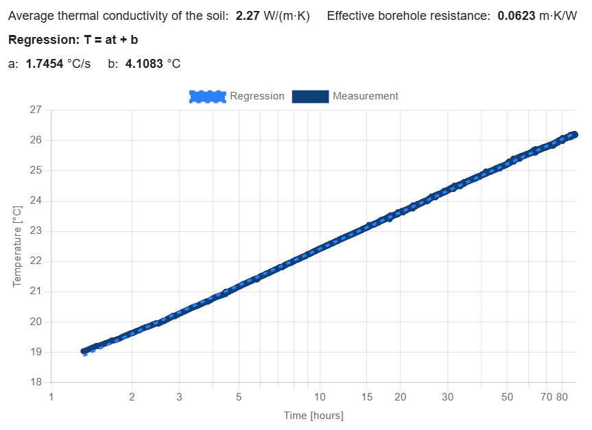
In the logarithmic plot, the mean fluid temperature increases more or less linearly after 10 hours. This is the linear behaviour described in the formula above, which only becomes visible in this so-called semi-log plot. Based on the data points from hour 10 to 60, a logarithmic approximation can be drawn. The slope of this line determines the k-factor in the formula above, and the intersection of this line with the y-axis determines the m-factor. From the following two equations, the ground thermal conductivity and effective borehole thermal resistance can be derived.
$$\lambda = \frac{\dot{Q}}{4\pi H k}$$ and $$R_b^*=\frac{H}{\dot{Q}}\cdot(\overline{T}_f(t)-T_0)-\frac{1}{4\pi \lambda}\cdot \left[ ln(t)+ln \left(\frac{4\alpha}{r_0^2}\right)-0.5772\right]$$
There is one parameter in this equation, $\alpha$ (the thermal diffusivity), that is strictly speaking also unknown, as it depends on both the thermal conductivity and the volumetric heat capacity of the ground. Since the thermal conductivity is typically searched for, this volumetric heat capacity has to be estimated based on literature for the geological conditions of your project and typically has a smaller influence than the other parameters (see for example table in Part 1.3).
There are other mathematical methods to analyse a TRT like the geostatistical analysis (GA-TRT) that estimates the thermal properties based on geostatistics and fluctuation data analysis (Focaccia et al., 2013).
Analyse a TRT in GHEtool Cloud
It is possible to analyse your thermal response test data in GHEtool Cloud an extract the parameters of interest. Below, the general settings, measurement data requirements and the results are discussed.
General settings
As explained in the methodology above, a few input parameters are required to perform the analysis:
- Volumetric heat capacity of the ground
In order to calculate the ground thermal conductivity with a TRT, an estimate of the volumetric heat capacity is required. This can be done based on the geology at the project location and by using tables with general thermal properties (see Part 1.3 for more information). - Borehole diameter and borehole length
Since the ILS model uses the specific heat injection (that is, the amount of power exchanged with the ground per unit length), both the borehole length and the borehole diameter are required. - Undisturbed ground temperature
As mentioned earlier, before the actual TRT measurement starts, the fluid can be circulated through the borehole without switching on the heating element. This allows the user to determine the initial undisturbed ground temperature, which is needed for the analysis of the TRT.

Measurement data
Depending on the data logger you use, the acquired data set might look slightly different (for example, some TRT machines also measure the flow rate and pressure drop through the system). The information that should always be provided, in one way or another, is:
- Time
To perform the analysis, a time series (in seconds) is required. - Power
It is important to know what (constant) power is injected into the ground. This power can either be entered manually as a constant or, if included in the measured data set, it can be extracted from that. - Fluid temperature
To understand how the borehole reacts to the injected power, the measurement of the fluid temperature is required. This can be done by providing both the inlet and outlet fluid temperatures or by using the average fluid temperature directly.
Results of the TRT analysis
The TRT analysis is rather straightforward and provides both the ground thermal conductivity and the effective borehole thermal resistance. In addition, the measurement data and the linear regression are shown, allowing you to check how well the model aligns with the measurements. If, for example, the regression deviates in the first part of the measurement, it could indicate that the borehole was not fully in steady state, and it is advised to increase the start index. An example of the regression graph is shown below.
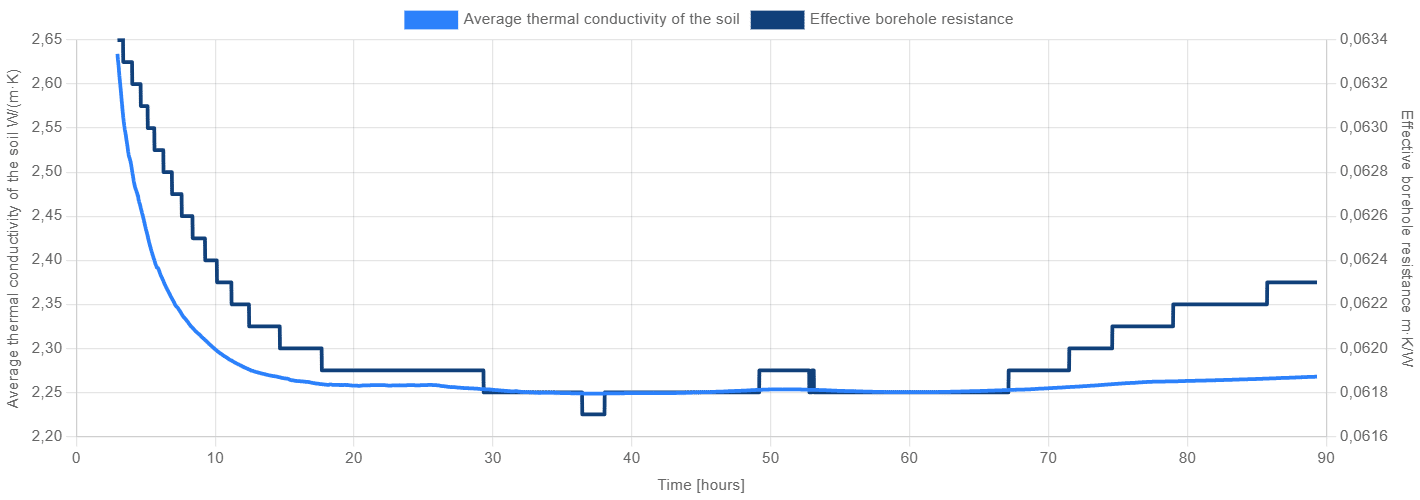
In order to know if your measurement period was long enough, a convergence graph is also shown. This graph increases the study horizon stepwise from considering only the first hour, the first two hours, the first three hours etc. until the whole measurement period has been considered. In the end, the values for the borehole resistance and the ground thermal conductivity should converge to a constant value. An example of a good convergence is shown below.
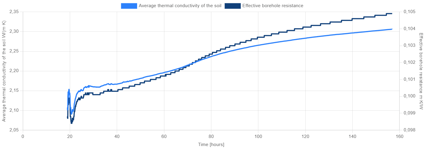
Below, an example is shown of a TRT that is not yet fully converged as can be seen by the increasing conductivity that has not yet reached a steady-state condition. This can either mean that the measurement period was not long enough, but it could also indicate the presence of a (significant) groundwater flow. Since the conductivity keeps rising in the figure below, the latter is probably the explanation (Sanner et al., 2008).
Use TRT results for your borefield design
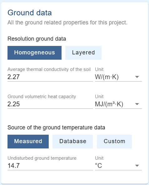
The results from a TRT can be used to simulate your borefield with greater accuracy. All the derived parameters can be entered directly into the software. In the example above, the results were:
- Undisturbed ground temperature: 14.7°C
- Ground thermal conductivity: 2.27 W/(mK)
- Effective borehole thermal resistance: 0.0623 mk/W
The first two parameters can be entered under the ‘Ground’ tab like in the figure below.
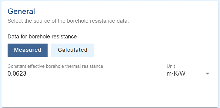
The effective borehole thermal resistance can be entered in the ‘Borehole resistance’ tab by setting the resistance data to ‘measured’, as shown in the figure below.
It is important to note that the measured effective borehole thermal resistance may not always be representative of the resistance you will have in your final project. Typically, a TRT is carried out without any antifreeze and with a flow rate that may differ from your design flow rate. In addition, a TRT is usually performed under heat injection conditions, whereas the most critical borehole resistance often occurs at the lowest temperature (as discussed in Part 3.2).
It is therefore recommended to always check the boundary conditions of the TRT to ensure they are applicable to your final design. If this is not the case, you can better rely on the borehole thermal resistance calculated by GHEtool instead.
Conclusion
In this chapter the Thermal Response Test (TRT) was discussed. This test can be used to obtain accurate measurements of both the ground properties (thermal conductivity and undisturbed ground temperature) as well as the effective borehole thermal resistance. In addition to the theoretical background and analysis via the infinite line source model, an example using GHEtool Cloud was presented. It was shown that the measurement of the effective borehole thermal resistance should be handled with caution, as it may not always be representative of the final project conditions. In such cases, it is preferable to calculate the effective borehole thermal resistance rather than relying solely on the measurement.
References
- Aydin, M., Onur, M., Sisman, A. (2019). A new method for analysis of constant-temperature thermal response tests, Geothermics, Volume 78, 1-8, https://doi.org/10.1016/j.geothermics.2018.11.001.
- Aydin, M., Dolcek, A.O., Onur, M., Sisman, A. (2024). Flow-controlled thermal response test and its comparison with the conventional test methods, Geothermics, Volume 120, 103011, https://doi.org/10.1016/j.geothermics.2024.103011.
- Jia, J., Lee, W.L., Cheng, Y. (2019). Constant-temperature thermal response test (TRT) with both heat injection and extraction for ground source heat pump systems: Methodology and a case study, Energy Procedia, Volume 158, 797-802, https://doi.org/10.1016/j.egypro.2019.01.210.
- Serageldin, A.A., Nagano, K. (2024). A novel oscillatory thermal response test method for efficient characterization of ground thermal properties: Methodology and data analysis, Renewable Energy, Volume 230, 120674, https://doi.org/10.1016/j.renene.2024.120674.
- McDaniel, A., Tinjum, J., Hart, D.J., Lin, Y.F., Stumpf, A., Thomas, L. (2018). Distributed thermal response test to analyze thermal properties in heterogeneous lithology, Geothermics, Volume 76, 116-124, https://doi.org/10.1016/j.geothermics.2018.07.003.
- Franco, A., Conti, P. (2020). Clearing a Path for Ground Heat Exchange Systems: A Review on Thermal Response Test (TRT) Methods and a Geotechnical Routine Test for Estimating Soil Thermal Properties, Energies, 13(11), 2965, https://doi.org/10.3390/en13112965.
- Gehlin, S. (2002). Thermal Response Test Method Development and Evaluation. Doctoral Thesis, Luleå University of Technology, Luleåtekniskauniversitet, Luleå.
- Focaccia, S., Tinti, R., Bruno, R. (2013). A software tool for geostatistical analysis of thermal response test data: GA-TRT, Computers & Geosciences, Volume 59, 163-170, https://doi.org/10.1016/j.cageo.2013.06.003.
- Sanner, B., Mands, E., Sauer, M.K., Grundmann, E. (2008). Thermal Response Test, A Routine Method To Determine Thermal Ground Properties For GSHP Design, 9th International IEA Heat Pump Conference, 20 – 22 May, Zürich, Switzerland