
Often, borefields are designed using standard configurations (rectangle, L-shape, etc.), although in reality the configuration is seldom that organised. In this chapter, we will discuss the importance of working with real borefield coordinates when designing your next geothermal project and the effect this has on the results and sizing.
Importance of working with irregular configurations
Although working with regular configurations is a fast and easy way to estimate the number of boreholes, it is not always representative of where the boreholes will actually be drilled. Chances are that the boreholes will be scattered around the building and positioned between pre-existing underground structures. Especially for large projects, the final borehole coordinates will often deviate from the assumed grid.
In order to illustrate this, an example in GHEtool will be presented using a building with a heating demand of 58 kW and a cooling demand of 30 kW, with associated yearly energy demands of 133 MWh/year and 38 MWh/year respectively. A double DN32 U-tube will be used with 25 v/v% MPG and a variable flow rate using a constant temperature difference of 4°C for both extraction and injection. The initial borefield configuration consists of a rectangular grid of 3 × 5 boreholes, spaced 5 m apart and 150 m deep. The temperature profile can be found below.
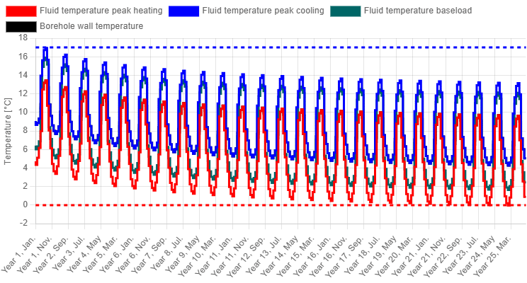
As can be seen in the graph above, there is a very strong imbalance towards extraction, cooling the borefield down year after year to -0.05°C. The maximum average fluid temperature in this case is 16.95°C.
When considering only regular configurations, the story would end with the simulation above, which represents a perfectly sized borefield. However, the boreholes in this project are not so well aligned and instead form a very irregular pattern, as can be seen in the figure below.

When the borefield is simulated using this irregular configuration, the following temperature profile is obtained.
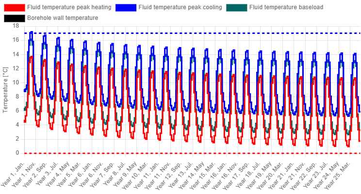
Here, the minimum average fluid temperature is significantly higher than in the case of the rectangular borefield (0.96°C), whereas the maximum average fluid temperature is only slightly higher at 17.21°C. The reason for this can be explained by the g-function concept, as discussed in Part 2.3. Every borefield configuration has its own unique g-function that describes its long-term behaviour and, since both configurations are rather different, different long-term behaviour can be expected.
The difference between the rectangular and the real irregular borefield configuration can also be illustrated using a temperature contour plot. Here, the temperature distribution in the ground caused by the imbalance is shown. Below, the situation for the rectangular grid is presented.
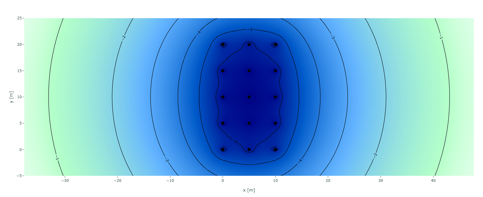
In the plot above, the cold is effectively trapped inside the borefield, with the ground temperature at the centre of the system decreasing by 6.5°C over a period of 25 years. When the real borehole coordinates are used, the situation is slightly different, as shown below. Here, due to the configuration, the cold region is spread out more, leading to a temperature decrease of only 5.5°C. This is therefore a two-dimensional representation of the same effect shown by the g-functions.

Since working with the real borefield configuration yields a more accurate result, it can reveal unnecessary oversizing. In the case above, the initial rectangular assumption was perfectly sized, but when the borefield was entered using the real coordinates, it was oversized. In fact, even when one borehole is removed, a minimum average fluid temperature of 0.26°C is still obtained. Hence, the required borefield size can be reduced by 6.7% just by calculating more precisely.
In the next two sections, it will be explained how to define a borefield with coordinates in GHEtool, using both a borehole map in AutoCAD and by creating the irregular grid directly in GHEtool Cloud.
Importing borehole coordinates from AutoCAD
Often, boreholes are planned by drawing them on a map in AutoCAD. These coordinates can easily be exported using AutoCAD’s DATAEXTRACTION feature into a CSV file that can then be imported into GHEtool Cloud. In this section, we will guide you through the different steps involved in this process. First, we will focus on the AutoCAD part, followed by the GHEtool part.
Export coordinates in AutoCAD
1. Open the DWG file containing the coordinates in AutoCAD.
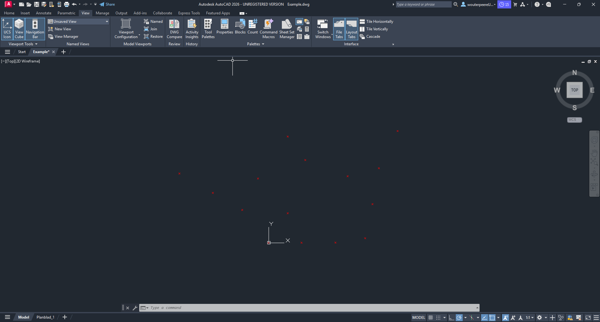
2. Select the coordinates you want to export.
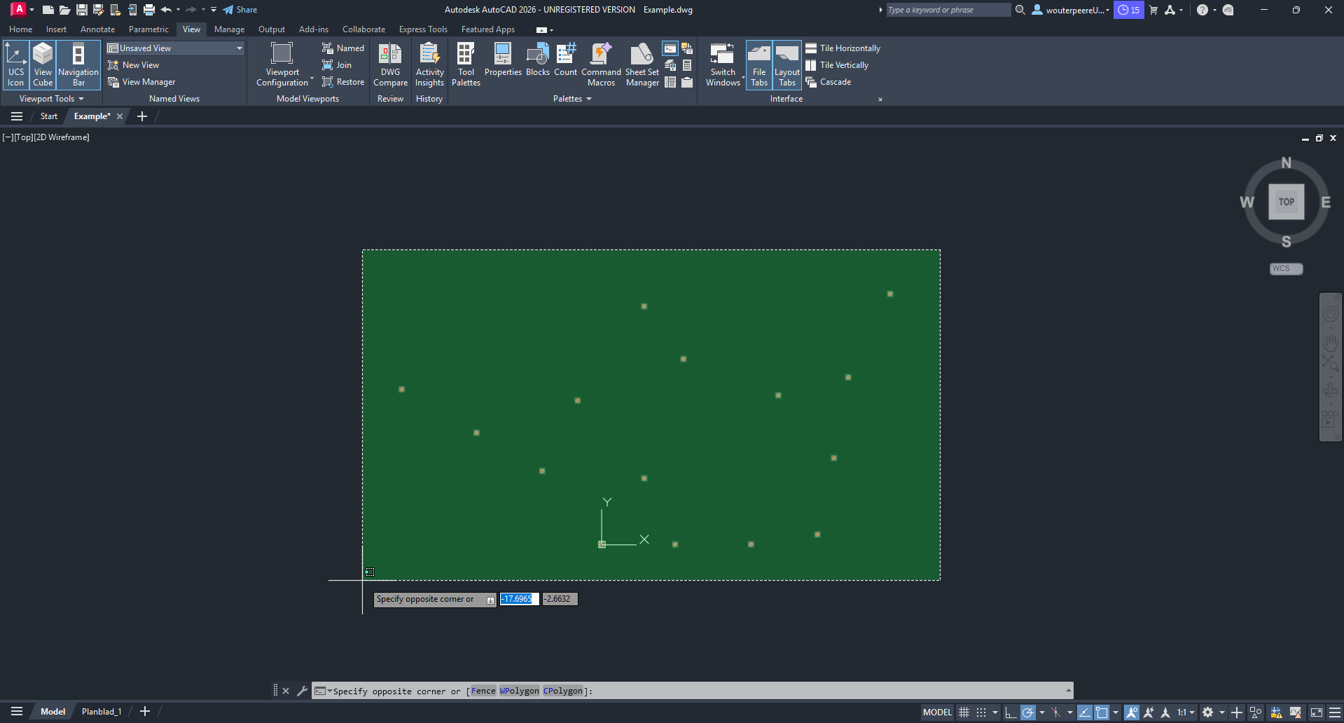
3. Type DATAEXTRACTION in the command line to open the Data Extraction dialogue box.
4. Select Create a new data extraction and press Next. A pop-up window will appear where you can choose a location to save the data extraction file. You can delete this file afterwards, as it is not required by GHEtool.
5. On the next screen, select Drawings/Sheet set.
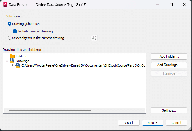
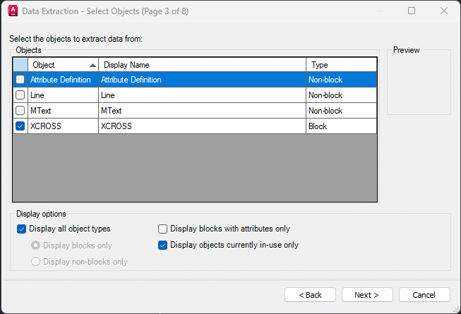
6. In Step 3, you are asked from which objects you want to extract the data. In this case, only XCROSS is required. All other irrelevant objects can be deselected.
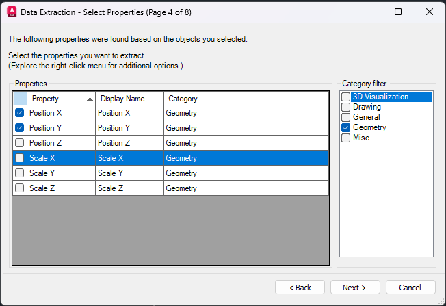
7. For each object, AutoCAD stores a considerable amount of information. However, we are only interested in the geometrical properties, namely the X and Y coordinates.
8. In the next step, the data can be refined. We do not need the Name or Count columns, so both can be deselected such that only the X and Y coordinates remain.
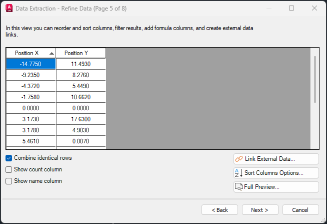
9. In Step 6, select Output data to external file and choose where you want to save the file. It is important that the file is exported as a CSV file.
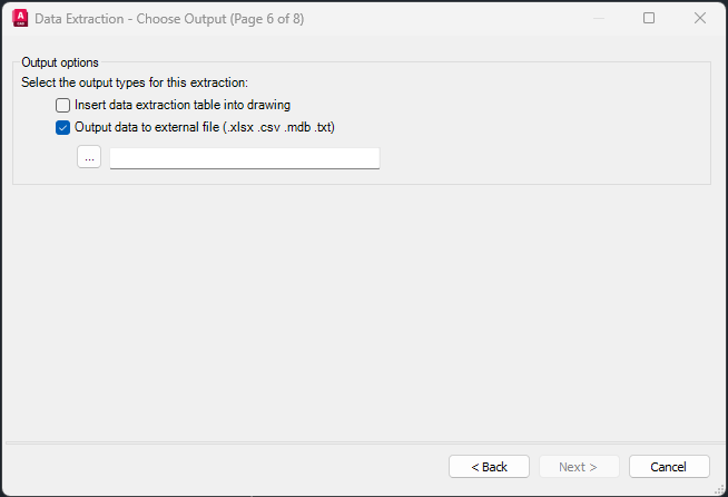
10. Click Finish, and the borehole coordinates will be exported to a CSV file.
In the next step, we will show you how to import these AutoCAD coordinates directly into GHEtool Cloud.
Import coordinates in GHEtool Cloud
Back in GHEtool, go to the Borefield tab and select Customized. In the Borefield inputs section, you can define your own borefield based on coordinates.
GHEtool Cloud offers three levels of custom borefield modelling:
- All borefields have the same depth and buried depth. This gives two degrees of freedom for each borehole: x and y position.
- Each borehole has its own depth and/or buried depth. This gives four degrees of freedom: x, y, depth, and buried depth.
- Each borehole can have its own tilt and orientation. This gives six degrees of freedom: x, y, depth, buried depth, tilt, and orientation.
Depending on which level you want to model, you will need to include the appropriate columns in your CSV file. For example, if you exported only the x and y positions from AutoCAD but want each borehole to have a different depth, you must manually add the column related to the borehole depth to the file.
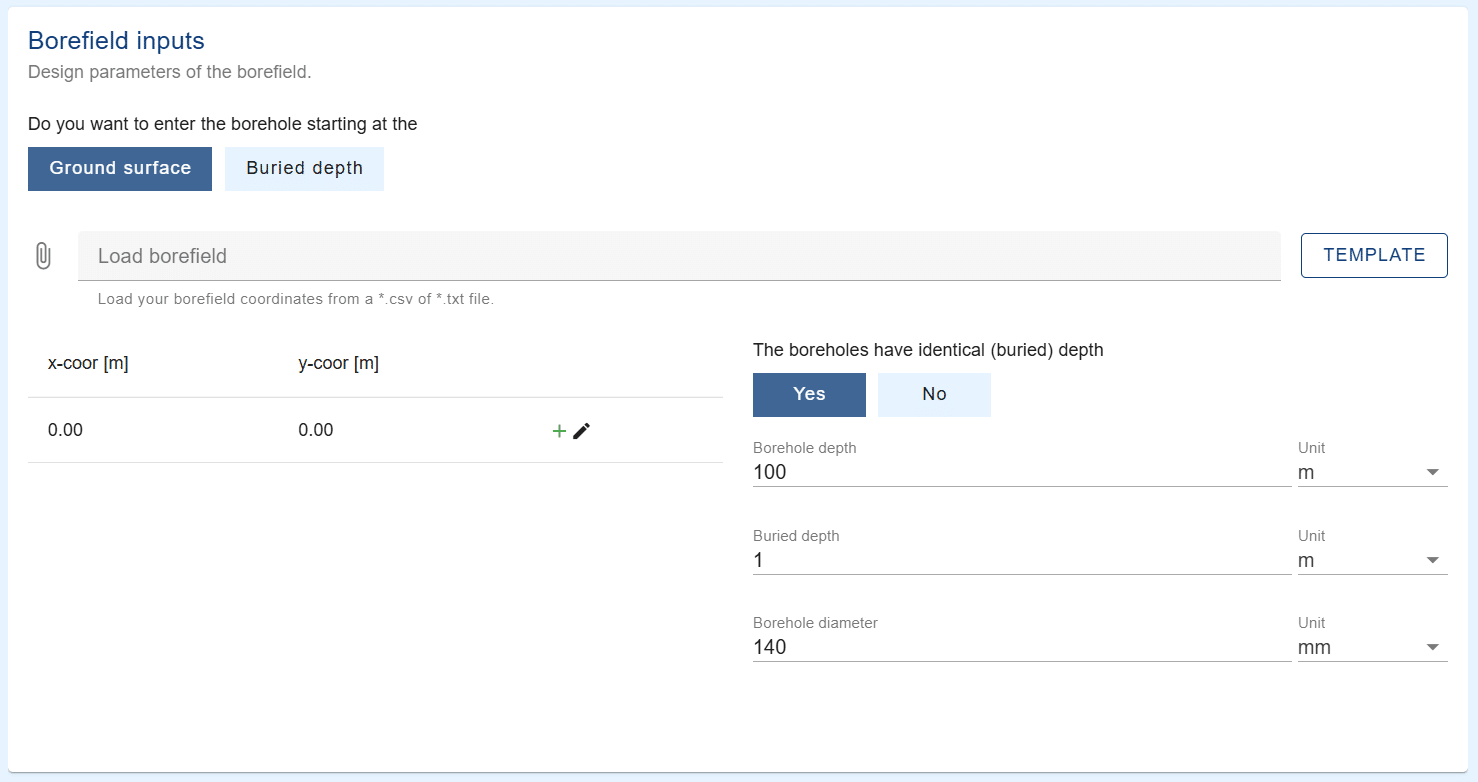
To import the coordinates, simply click on Load borefield and select your CSV file. Afterwards, you will be asked to link the columns to the correct data inputs and specify the units.
Once this is done, two options are available for importing the data:
- Overwrite existing borefield: this will remove all coordinates currently present and replace them with those from the file.
- Add to existing borefield: this will add the coordinates from the file to the coordinates already present.
Creating irregular configurations in GHEtool Cloud
In case you do not have an AutoCAD file, it is possible to create irregular configurations directly in GHEtool. This can be done by going to the Customized borefield and duplicating boreholes by clicking the + icon in the borehole list or by clicking on a borehole in the plot at the bottom of the screen.
However, an irregular configuration often starts from a layout that is more or less regular. For example, imagine you want to create a borefield with 17 boreholes. This could easily be achieved by starting with a 3 × 6 grid and removing one borehole. However, entering all these boreholes manually is rather time-consuming. Therefore, you can start with a rectangular configuration, or any other regular configuration, and click on a borehole in the chart below. You will then be asked whether you want to convert the current borefield into a manual one. Once this is done, the borefield will be defined using its coordinates and you can add or remove boreholes individually.
Bulk operations
Sometimes, you may want to perform bulk operations on a borefield, such as moving the entire borefield or rotating it. This can be done by clicking on the Options button in the top right corner of the borefield plot and selecting either Move borefield or Rotate borefield.
Move borefield
If you want to move the borefield, you simply need to define one coordinate in the current reference frame and the corresponding coordinate in the new reference frame. For example, if you want to move the entire borefield 30 m to the right, you can move the coordinate (0,0) to (30,0). This will shift all boreholes 30 m to the right.
Rotate borefield
If you want to rotate the borefield, you need to define a point around which the borefield should be rotated. Imagine the origin is at (0,0) and you want to rotate the borefield around this point by 90° clockwise. In that case, you would set (0,0) as the rotation point and rotate point (0,1) to (1,0). This will rotate the entire borefield by 90° clockwise.
Work on a map
One final feature in GHEtool related to custom borefield configurations is the ability to draw coordinates directly onto a map. This not only provides additional visual information about the location of the boreholes, but also makes it easier to position them using drag-and-drop.
To do this, click on the Background button in the top right corner of the borefield plot, again within the Customized borefield tab. The pop-up window is shown below.
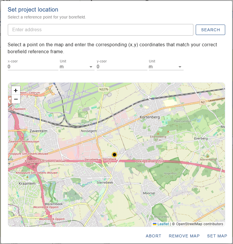
Since coordinates on a map are typically given as longitude and latitude, whereas borehole coordinates are generally defined using Cartesian x and y coordinates, a way is needed to connect the two systems. This is done by clicking on the map to define a reference point. For this reference point, you need to enter the x and y coordinates corresponding to that location. In this way, the local coordinate system in which the borefield is drawn will be correctly positioned on the map.

In the image above, the boreholes are visible on the map and can easily be dragged and dropped into the correct locations. The positions in the coordinate list above will automatically be updated as well. By double-clicking on the map, additional boreholes can easily be added to the system, making it fast and straightforward to create even the most complicated borefield configurations in just a few clicks.
Conclusion
In this chapter, it was shown how borehole coordinates can be used to define an actual borefield in GHEtool. It was explained how coordinates drawn on a map in AutoCAD can be exported to a CSV file and later imported into the tool. In addition, it is also possible to create a custom borefield directly in GHEtool, either from scratch or by starting from a regular grid. When positioning boreholes on a map, it becomes even easier to move them around.
Working with the exact borehole coordinates was shown to provide valuable insights and can help avoid oversizing of a geothermal system. In the example discussed, 1 out of 15 boreholes could be removed simply by modelling the borefield more accurately.
In the next section, we will conclude this part by discussing different ways to cope with imbalance in geothermal design.