
In this chapter, the modelling of the TurboCollector from MuoviTech is explained, together with a broader explanation of computational fluid dynamics and the concept and importance of turbulence.
TurboCollector
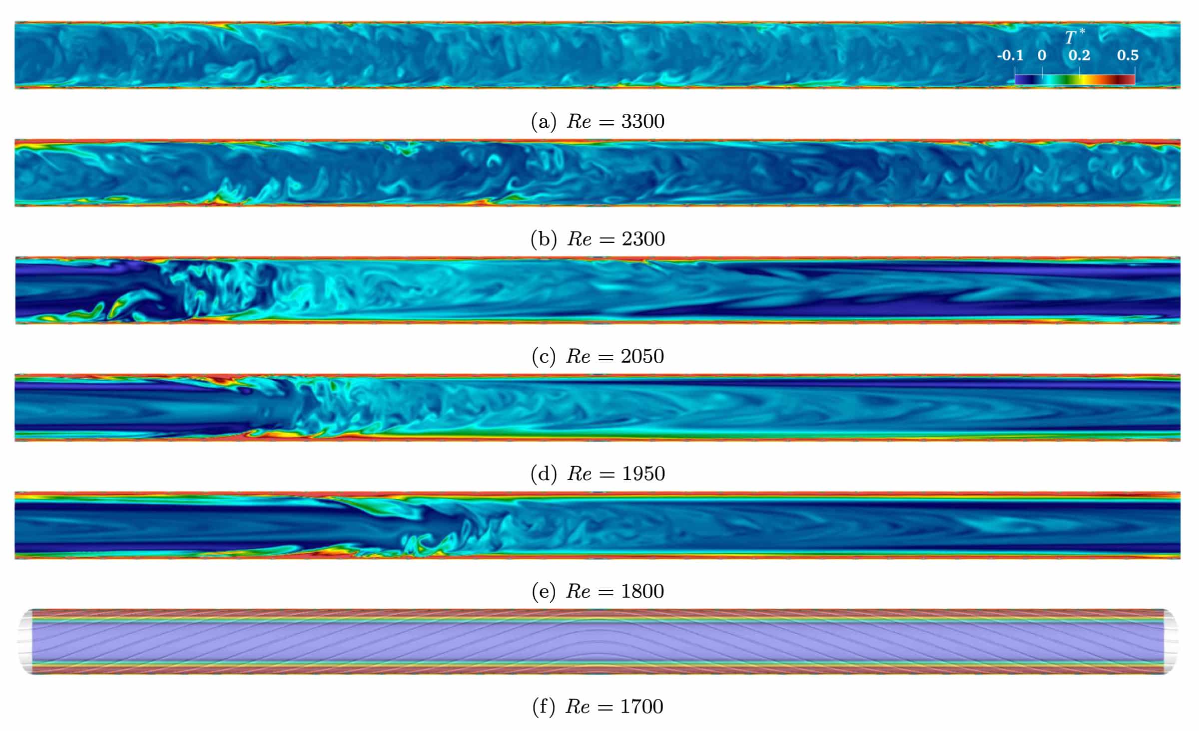
The TurboCollector is a product developed by MuoviTech which, unlike traditional smooth pipes, features multiple small fins along its inner surface. These fins are oriented in alternating clockwise and counterclockwise directions along the length of the pipe, acting as passive turbulators. They are designed to induce turbulent flow behaviour at lower flow rates, thereby enhancing heat transfer. In standard smooth pipes, the transition to turbulence typically begins at a Reynolds number of around 2300, but with the TurboCollector’s internal geometry, turbulence is initiated at approximately Re = 1700 to 1800.

However, quantifying the effect of the internal fins on both the thermal and hydraulic behaviour is not straightforward, which is why the challenge of turbulence simulation and computational fluid dynamics is introduced in the next section. After that, the actual pipe modelling is explained.
Turbulence modelling and CFD
Computational Fluid Dynamics (or CFD for short) is one of the most important fields in engineering today. It is used to simulate fluid behaviour in chemical plants, optimise the shape of aircraft wings to maximise lift, assess the aerodynamic performance of vehicles, predict wind turbine output, and much more. Below, an image of a CFD simulation of an aircraft wing is shown. When it comes to modelling the thermohydraulic behaviour of the TurboCollector, CFD is the preferred method.

Although CFD simulations are widely used, accurately modelling turbulence remains extremely challenging. Turbulence (as discussed in Part 2.2, when the Reynolds number was introduced) is a highly chaotic state of fluid motion for which no analytical solution exists. This is because turbulence occurs across a wide range of both temporal and spatial scales. For instance, when an aeroplane flies through a cloud, you might observe large scale vortices in the cloud and, within those, even smaller swirling structures, and so on. To fully capture this turbulent behaviour, simulations must resolve all the way down to the finest scales.
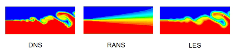
In the literature, three main approaches are commonly used to simulate turbulence, all of which are illustrated below.
- RANS (Reynolds-Averaged Navier-Stokes)is the fastest but least accurate approach. As shown in the figure, the fine scale vortices are completely smoothed out, making this method unsuitable for modelling the TurboCollector, since the small scale turbulence is not modelled explicitly.
- LES (Large Eddy Simulation) is a more advanced method that distinguishes between large scale and small scale turbulence. The larger eddies are resolved directly, while the smaller scale turbulence is modelled. This approach is typically a good compromise, as some flow structures become visible, but it is still not suitable for modelling the subtle turbulence regions in the TurboCollector.
- DNS (Direct Numerical Simulation) is the most accurate, but also the most computationally intensive, method for simulating turbulence, as it solves the fluid equations numerically over extremely small time and spatial intervals. The figure clearly shows that this method provides the most detailed and realistic representation of turbulence and is therefore ideal for modelling the TurboCollector.
All fluids, whether water, air or any other fluid, are governed by the Navier Stokes equations. This equation, given below solely for its beauty, is the following:$$\rho \frac{D\vec V}{Dt}=-\nabla p + \rho \vec g + \mu \nabla^2 \vec V$$ This equation is notoriously complex to solve, which is why, even today, after more than 200 years, no analytical solution exists. This is why we rely on computationally intensive numerical methods such as DNS to solve it numerically.
The importance of this problem is so significant in physics that a one million dollar prize has been offered to anyone who can solve it. You can find more information on this challenge here.
In the following section, the thermohydraulic simulation of the TurboCollector is explained based on this highly detailed DNS method.
Model development
In order to provide a baseline case that can later be used as a reference for the TurboCollector, a smooth pipe was first simulated using the DNS approach. The result is shown below.
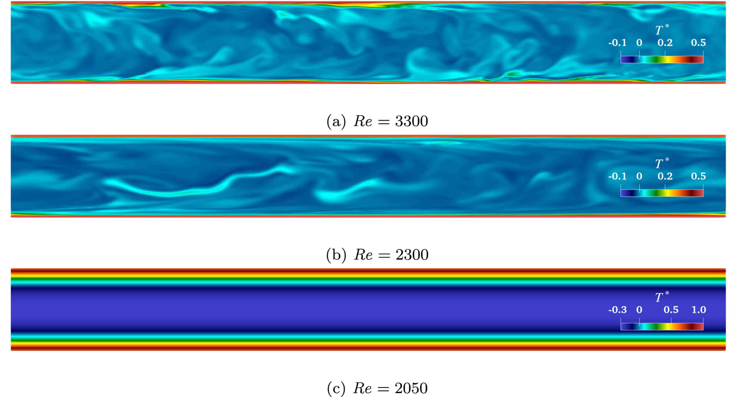
In order to determine the onset of turbulence, the pipe is first simulated at a very high Reynolds number, where the flow is definitely turbulent. This is also clearly visible in the figure above, where the fluid is rather homogeneous in colour, with only a small boundary layer at the pipe wall, indicating a turbulent flow regime. When the Reynolds number is lowered to Re = 2050, the laminar regime becomes clearly visible, with distinct layers near the pipe walls. Here, the temperature difference between the inner fluid layers and the outer ones is more pronounced, which is why heat transfer in the laminar regime, as discussed before, is less effective.
In the simulations above, the concept of the boundary layer is clearly visible. This is the region between the pipe wall and the distance from the wall where the flow velocity approaches the bulk velocity of the fluid, defined as the flow rate divided by the cross sectional area.
In the laminar regime, the viscous forces between the fluid particles are dominant and the particles literally drag each other along. This results in a very thick boundary layer which, in turn, leads to lower heat transfer. In the figure below, the velocity profile is shown for this laminar case (on the left), where it is clearly visible that the velocity increases gradually towards the centre of the pipe.
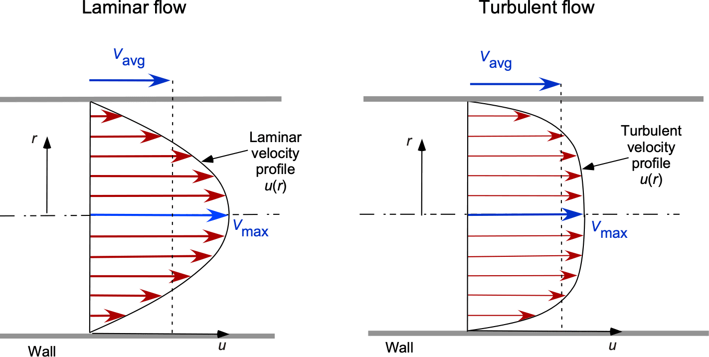
In contrast, the velocity profile in the turbulent regime increases much more rapidly when moving from the pipe wall towards the centre of the pipe. This results in a very steep velocity gradient at the pipe wall and, consequently, a thinner boundary layer. This is why, in the simulations above, the width of the colour gradient was smaller for the turbulent case than for the laminar case.
The figure below shows the same simulation for the TurboCollector. The story is the same for Re = 3300, where the flow is also turbulent, just as in the smooth pipe. When the flow rate is reduced, and hence also the Reynolds number, the flow remains rather well mixed. It is only at around Re < 1800 that a distinct boundary layer starts to form, which is why Hidman et al. (2026) concluded that the transition region starts at Re > 1700, which is significantly lower than for a smooth pipe.
Given the simulation results above, two important correlations can be derived: one for the friction factor, which is important for the pressure drop, and one for the Nusselt number, which is important for the convective heat transfer. Both are discussed below.
Correlation for the friction factor
In the graph below, the friction factor of the TurboCollector (indicated as ‘Alternating DNS’) is plotted against the analytical friction factor correlations for both the laminar and turbulent regimes.
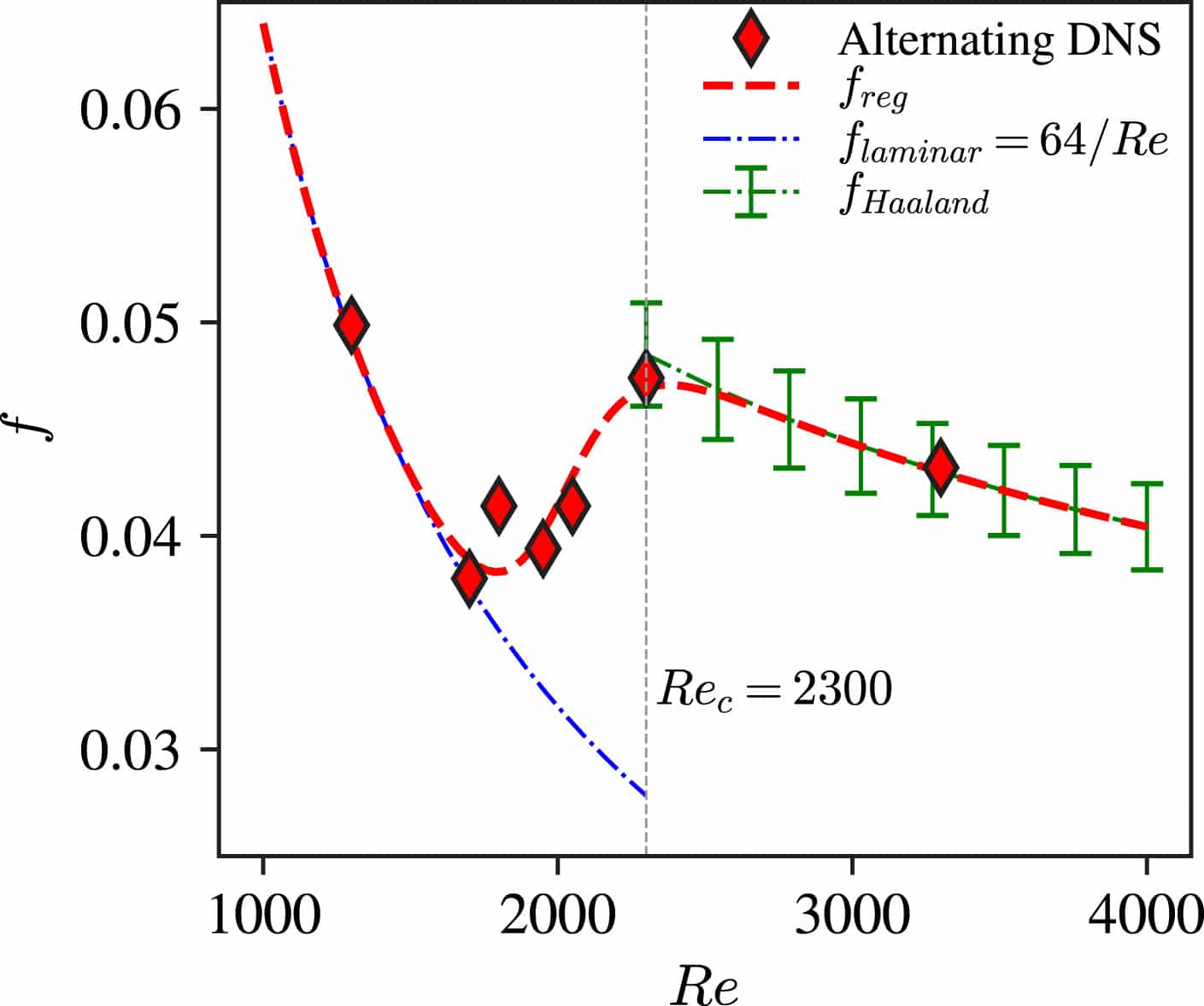
It is clear that the friction factor follows the analytical solution for a smooth pipe quite well at lower Reynolds numbers, but it starts to deviate at around Re = 1700 to 1800, where the flow begins to become turbulent due to the internal fins. Once the Reynolds number reaches 2300, both the TurboCollector and the smooth pipe are fully turbulent and their friction factors are more or less identical.
Correlation for the Nusselt number
In the figure below, the Nusselt number is plotted as a function of the Reynolds number.
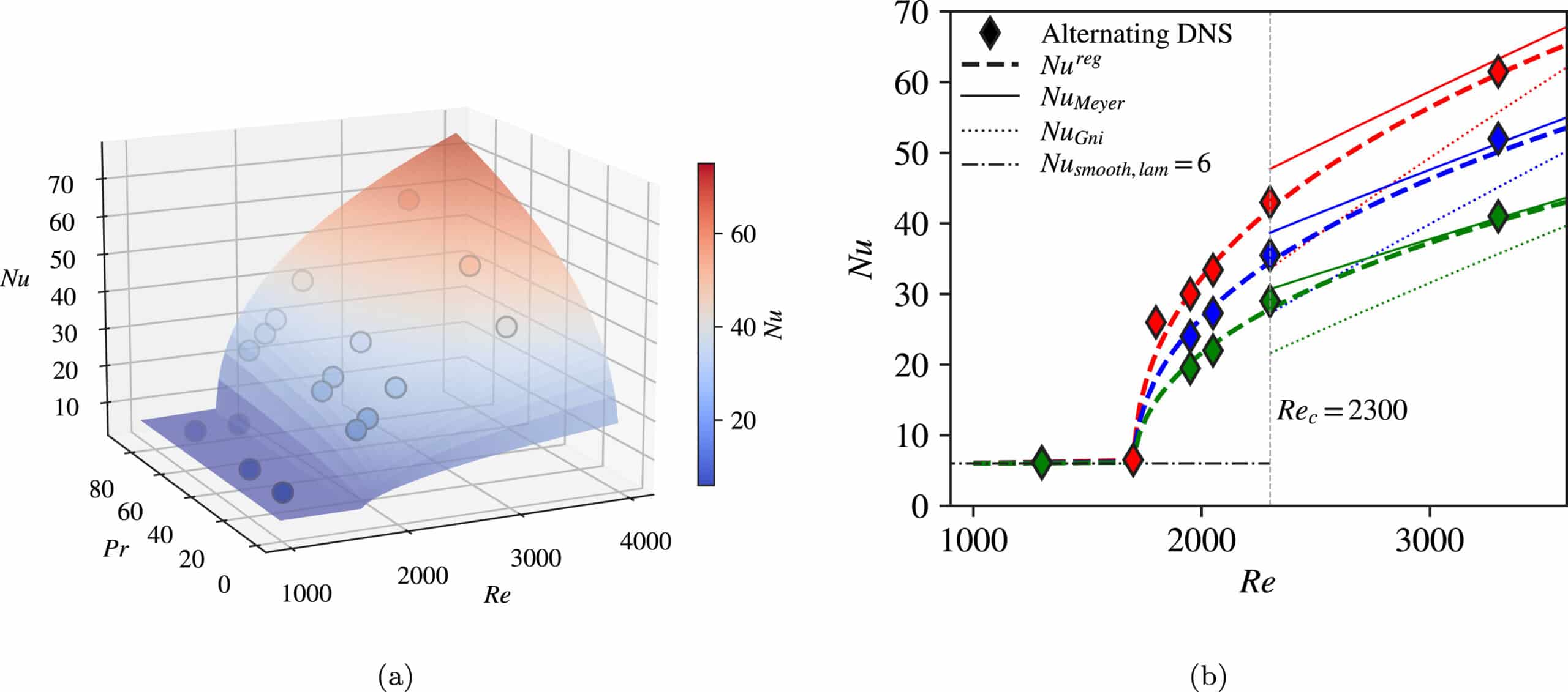
Since the Nusselt number is now plotted as a function of both the Reynolds number and the Prandtl number (green: 20, blue: 40, red: 75), the correlation forms a surface, as shown in the figure above (left). On the right, the corresponding correlations are shown, where the transition region again starts at Re = 1700 and increases rapidly afterwards. At Re = 2300, when the smooth pipe becomes turbulent, the TurboCollector still has a slight advantage, but this gradually disappears towards fully turbulent flow (Re = 4000), where the Nusselt numbers for the smooth pipe and the TurboCollector are almost identical.
Since the highest Reynolds number considered in the DNS simulations was 3300, the correlation above has not been validated beyond this range. However, as can be seen from the graphs, it converges towards the Gnielinski correlation at around Re = 4000. Therefore, in GHEtool, this correlation is used up to Re = 4000. For Re > 4000, the Gnielinski correlation for the Nusselt number is used, with a constant offset $\delta$ to account for the effect of the fins at higher Reynolds numbers. This offset is defined as:$$\delta = Nu_{Gnielinksi}(4000)-Nu_{TurboCollector}(4000)$$For the full mathematical details, the reader is referred to Hidman et al. (2026).
Behaviour of the TurboCollector
Given the two correlations developed above, the effective borehole thermal resistance and the pressure drop of the TurboCollector are discussed in the next sections.
Effective borehole thermal resistance
he graph below revisits the discussion of the single versus double U-tube from Part 5.1 but now includes the TurboCollector in the comparison.
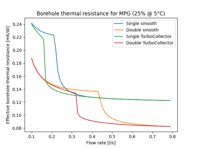
As you can see, the onset of the transition regime occurs earlier for the TurboCollector than for the equivalent smooth pipe, for both the single and double U-tube configurations. This means that, when the TurboCollector DN32 is compared with the smooth double DN32, the range in which the former performs better increases from 0.28 to 0.45 l/s to 0.18 to 0.45 l/s. This implies that you can achieve a lower borehole thermal resistance with a single U-tube at a lower flow rate.
Another way to take advantage of this earlier transition to turbulence is to use a slightly larger pipe diameter (DN40), as shown in the figure below.
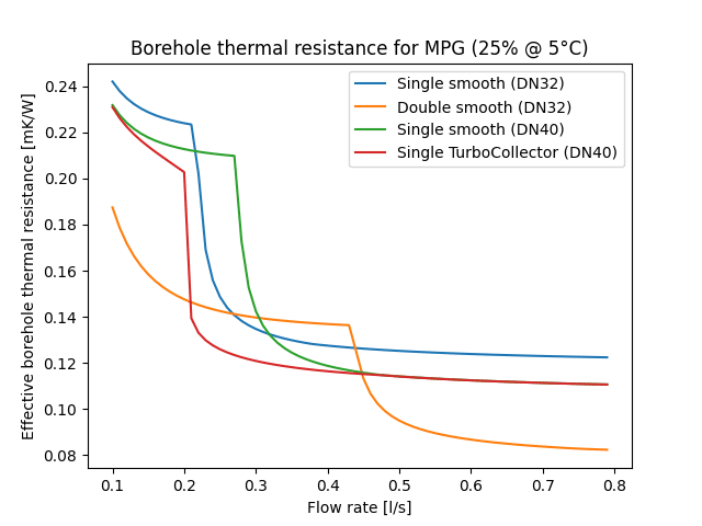
In Part 5.1, it was stated that a single DN40 has a shorter range in which it outperforms a double DN32, but that the reduction in borehole thermal resistance is more pronounced than when comparing a single DN32 with a double DN32. When the TurboCollector DN40 is added to the comparison, the range in which the DN40 outperforms the double DN32 doubles from 0.3 to 0.45 l/s to 0.2 to 0.45 l/s. This provides another way of looking at the same problem.
Pressure drop
Besides the thermal aspects discussed above, the pressure drop is also important. In the figure below, the hydraulic aspects of the single versus double U-tube discussion from Part 5.2, are revisited.
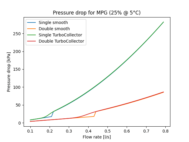
In the figure above, it is again clear that the single DN32 has a significantly higher pressure drop than the double U-tube at the same flow rate. Since the transition to turbulence starts earlier in the TurboCollector, a clear increase in pressure drop is visible compared with the smooth pipe. This is the price paid for the increased turbulence. However, in both the laminar and turbulent regimes, the TurboCollector performs very similarly to the smooth pipe, with only a 2 to 3% higher pressure drop. This is in line with the correlation above, which converges to the friction factor of the smooth pipe in both the laminar and turbulent regimes.
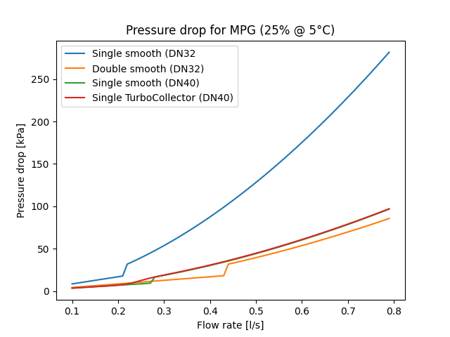
In the graph above, the hydraulic counterpart of the thermal comparison above is shown. Here, the single DN40 (both smooth and TurboCollector) is compared with the single DN32 and the double DN32. It is clear that, as discussed in Part 5.2, the single DN32 is by far the worst option, while the other three perform similarly, with the DN40 probes outperforming the double DN32 at very low flow rates.
Conclusion
In this chapter, the TurboCollector from MuoviTech was introduced. First, the importance of turbulence modelling was explained by introducing both computational fluid dynamics and the direct numerical simulation methodology to resolve the flow regime down to the finest turbulence scales. Using this type of thermohydraulic simulation, it was found that the transition to turbulence starts at around Re ≈ 1700.
When looking at the effective borehole thermal resistance, the TurboCollector offers a wider operating range in which the flow remains turbulent, or at least transitional, meaning that it extends the range in which a single U-tube outperforms a double U-tube. From a hydraulic perspective, the pressure drop is very similar to that of a smooth pipe, except in the range Re = 1700 to 2300, where the improved heat transfer comes at the cost of a higher pressure drop.
References
- Hidman, N., Almgren, D., Johansson, K., Nilsson, E. (2026). How internal fins enhance the thermohydraulic performance of geothermal pipes: A direct numerical simulation study, International Journal of Heat and Mass Transfer, Volume 256, Part 3, 2026, 128114, ISSN 0017-9310, https://doi.org/10.1016/j.ijheatmasstransfer.2025.128114
- Gordon Leishman, J. (2026). Introduction to Aerospace Flight Vehicles, part 29: Internal flows. Available online at: https://eaglepubs.erau.edu/introductiontoaerospaceflightvehicles/chapter/internal-flows/