Supabase, our database hosting service, has a global problem, due to which, GHEtool is not operational at the moment. You can follow the status on https://status.supabase.com/.

Back to overview

Ready to explore all possibilities of GHEtool Cloud?

Schedule a demo call

You can try GHEtool 14 days for free,
no credit card required.

Part 6
Chapter 3
June 2026
Wouter Peere

GEROtherm VARIO and FLUX

In this chapter, the modelling of the GEROtherm VARIO and FLUX probes from HakaGerodur is explained, together with the use of the mean value theorem to account for their conical geometry.

GEROtherm VARIO and FLUX

The GEROtherm® FLUX and VARIO probes are two innovative heat exchangers developed by HakaGerodur. They are designed to have the same pressure rating as a regular smooth geothermal probe, but with a lower pressure drop. To achieve this, the wall thickness of the probe is increased towards the bottom of the borehole, ensuring the required strength where the static pressure is highest. This design gives the VARIO and FLUX probes an overall larger inner diameter, which is beneficial for reducing the pressure drop. A vertical cross section of a FLUX probe is shown below.

From a modelling perspective, the GEROtherm VARIO and GEROtherm FLUX are both treated as conical pipes. However, FLUX probes are designed for very deep boreholes (up to 500 m), while VARIO probes are intended for shallower systems (up to 250 m).

Vertical cross section of the GEROtherm® FLUX 43DN PN32 probe.

More information on the GEROtherm VARIO and FLUX probes can be found, respectively, here and here.

Model development

In this section, the model development for the conical GEROtherm VARIO and FLUX probes is discussed.

One pipe, three regions

When we take a closer look at the VARIO and FLUX probes, we can see that they consist of three sections. The first section of the probe is a regular smooth pipe with a constant wall thickness, for which the solution is already known. The last section of the probe is also a regular pipe with a constant, but different, wall thickness. The section in between, where the wall thickness gradually increases, is where a new model needs to be developed.

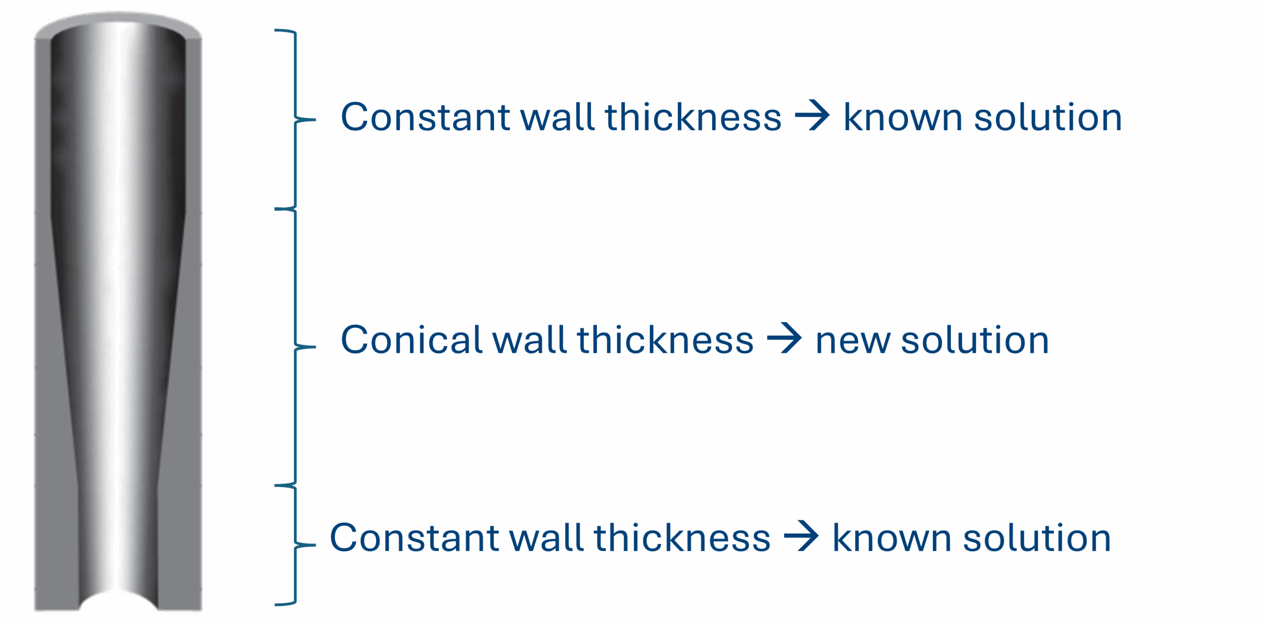
Some GEROtherm VARIO probes end immediately after the conical section and therefore do not include a final section with a constant wall thickness. This has no impact on the development of the model, since for these probes the final section simply has a fictitious length of zero.

The three different models for the conical probe design.

A first idea might be to simply take the average value of the relevant parameters (such as the Reynolds number, the friction factor and the borehole thermal resistance) between the start and end of the conical section. However, since these parameters do not vary linearly with the borehole depth (and the corresponding wall thickness), this does not provide a good estimate. A more accurate approach is to use the mean value theorem, which is discussed in the next section.

Mean value theorem

Typically, when calculating an average value, we take two values and divide their sum by two. This inherently assumes a linear relationship between those two values. However, when the relationship is far from linear, this is not a very accurate approach. Let us consider the red line in the graph below as an example.

Graphical illustration of the mean value theorem. — Graphical illustration of the mean value theorem. (source: https://www.statisticshowto.com/calculus-problem-solving/intermediate-value-theorem/mean-value-theorem)

In order to calculate the average value of the red line between $a$ and $b$, the following formula can be used:$$f(c)=\frac{1}{b-a}\int_a^bf(x)dx$$where $a$ and $b$ are the points between which the mean value should be taken (in our case, the beginning and the end of the conical section), $f(x)$ is the function for which the mean value should be calculated, and $f(c)$ is the actual average value. The idea is to find a rectangle with base $b-a$ and height $f(c)$ such that the area $(b-a)f(c)$ is equal to the area under the original graph.

At first, this may seem overly complicated. However, if we look at the graph of the Reynolds number in the conical section of the probes, we see a clear difference. Since we are working with long probes (up to 500 m for the GEROtherm FLUX), this difference can have a significant impact, especially in the transient region. The mean value theorem is therefore applied when calculating the Reynolds number, the friction factor, the pressure drop, and the effective borehole thermal resistance.

Difference between using the average value and the mean value theorem for the Reynolds number in the conical part.

It is also possible, using the mean value theorem, to derive analytical solutions for certain properties, such as the Reynolds number. If the conical section starts with an inner diameter of $D_{in,0}$ and the wall thickness increases at a rate $a$ in (m/m), the inner diameter at position $x$ (measured from the top of the conical section) can be calculated as:$$D_{in}(x)=D_{in,0}-2ax$$The Reynolds number is defined as:$$Re=\frac{\rho DV}{\mu}$$with $\rho$ the fluid density in (kg/m³), $D$ the pipe inner diameter in (m), $V$ the fluid velocity in (m/s), and $\mu$ the dynamic viscosity of the fluid in (Pa·s). Since we know that the flow velocity $V$ depends on the flow rate $\dot{V}$ in (m³/s) and the cross sectional area $A$, the Reynolds number can be rewritten as:$$Re=\frac{\rho D\dot{V}}{\mu A}=\frac{4\rho D\dot{V}}{\mu\pi D^2}=\frac{4\rho\dot{V}}{\mu\pi D}$$Using the position dependent inner diameter, the Reynolds number can be written as a function of the position $x$ in the conical section:$$Re(x)=\frac{4\rho\dot{V}}{\mu\pi D(x)}=\frac{4\rho\dot{V}}{\mu\pi(D_{in,0}-2ax)}$$Using the mean value theorem, the average Reynolds number $\overline{Re}$ can be calculated as:$$\overline{Re}(x)=\frac{1}{x-0}\int_0^xRe(x)dx=\frac{1}{x}\int_0^x\frac{4\rho\dot{V}}{\mu\pi(D_{in,0}-2ax)}dx$$Which gives:$$\overline{Re}(x)=\frac{-2}{x}\frac{\rho\dot{V}}{\mu\pi}\left[\ln(D_{in,0}-2ax)-\ln(D_{in,0}) \right]$$

Behaviour of the GEROtherm VARIO and FLUX

Using the model above, the effective borehole thermal resistance and the pressure drop of the GEROtherm VARIO and FLUX probes are discussed below.

All simulations below are performed using a borehole with a depth of 160 m and a buried depth of 70 cm. The borehole diameter is 140 mm, the grout thermal conductivity is 1.5 W/(mK), and the ground thermal conductivity is 2 W/(mK). The pipes are placed exactly halfway between the borehole centre and the borehole wall, i.e. at a distance of 35 mm from the borehole centre. The fluid used is MPG at 25 v/v% and 5°C. All pipes have a PN16 (SDR11) pressure rating and a thermal conductivity of 0.4 W/(mK). Unless stated otherwise, the pipe diameter is 32 mm. Any deviations from the assumptions above are explicitly mentioned below.

Effective borehole thermal resistance

Below, the effective borehole thermal resistance is shown for the regular single and double DN32 U-tubes and the VARIO DN32.

Please note that, in contrast to the other articles and the discussion in Part 5.1, the borehole depth below was set to 160 m, because it is only at this depth that the GEROtherm VARIO DN32 reaches the PN16 pressure rating. Any other borehole depth would have resulted in an unfair comparison in terms of pressure rating.

Effective borehole thermal resistance for single and double U-tube DN32, and a single and double GEROtherm VARIO DN32.

When it comes to the discussion of single versus double U-tubes, the use of a VARIO does not change much. It can be seen that the VARIO has a slightly lower borehole thermal resistance in both the laminar and turbulent regimes due to the, on average, slightly smaller wall thickness and hence the lower pipe thermal resistance.

In contrast, the transition to turbulence does not occur at a single flow rate, since the inner pipe diameter is no longer constant. It starts becoming transient at the same time as in the regular probes, but because the upper part of the VARIO has a larger inner diameter, a higher flow rate is required for the entire pipe to become transient or turbulent. This is why the transition to the transient regime is less pronounced for the conical probe.

The VARIO DN32 PN16 is the shallowest probe in the range. To illustrate a more common use case, a GEROtherm FLUX DN43 PN32 and a FLUX DN53 PN38 are simulated below for a borehole depth of 350 m and a borehole diameter of 170 mm. These are compared with a single and double DN40 PN32 U-tube.

Effective borehole thermal resistance for single and double U-tube DN40 PN32, and a singe FLUX DN43 PN32 and FLUX DN53 PN38.

In the graph above, the range in effective borehole thermal resistance is much more pronounced than in the previous two cases due to the greater borehole depth. The transition to the turbulent regime is now very clear for all pipes, including the conical ones, where the two different transition points (one for the smallest inner diameter and one for the largest) are clearly visible.

Also in this case of a deeper borehole, the single U-tube (FLUX DN43 and FLUX DN53) can outperform the double U-tube over a specific flow rate range. In the turbulent regime, towards the upper end of the graph (where most deep probes will operate), the single FLUX DN53 has a very similar borehole thermal resistance to the double U-tube, albeit slightly lower due to the smaller average wall thickness (PN38 instead of PN32).

So, from a thermal perspective, the conical probes perform very similarly to the regular ones, but with a slightly lower borehole thermal resistance (when the same diameters and pressure classes are compared) due to the, on average, smaller wall thickness. The major advantage of these systems, however, lies in their hydraulic performance.

Previously, it was stated that the convective heat transfer in the laminar regime is constant, given the constant Nusselt number of 3.66. One may therefore wonder why there is such a large variation in effective borehole thermal resistance within this laminar regime.

The reason lies in the way the effective borehole thermal resistance is calculated. In Part 2.2, it was explained that the thermal resistances inside the borehole are much more complex than just the fluid, pipe and grout resistances. Mathematically, two sub resistances are considered: the local borehole resistance ($R_b$), which expresses the resistance to heat transfer from all pipes to the borehole wall, and the internal resistance ($R_a$), which quantifies the heat transfer between the different pipes.

For a given pipe configuration, these two resistances are constant along the pipe length, since they are determined purely by the two dimensional cross section. However, the effective borehole thermal resistance is a function of the pipe length and is related to the other two resistances as follows:$$r_v=\frac{H}{\dot{m}_{pipe}C_p}$$ $$\alpha = \frac{r_v}{n\cdot R_b \cdot R_a}$$ $$R_b^*=R_b\cdot \alpha\cdot \coth(\alpha)$$where $H$ is the borehole length in (m), $\dot{m}_{pipe}$ is the mass flow rate per pipe in (kg/s), $C_p$ is the fluid heat capacity in (J/(kgK)), and $n$ is the number of pipes.

From the equations above, assuming a uniform average borehole wall temperature, the relationship between the effective borehole thermal resistance and the mass flow rate becomes clear. Even though both $R_a$ and $R_b$ remain constant in the laminar regime, increasing the flow rate decreases $r_v$ and therefore also decreases the effective borehole thermal resistance.

Pressure drop

In the figure below, the hydraulic counterpart to the comparison between the regular single and double DN32 U-tubes is shown, together with the GEROtherm VARIO DN32 probe.

Effective borehole thermal resistance for single and double U-tube DN32, and a single and double GEROtherm VARIO DN32.

It is clear that, at all flow rates, the VARIO probe outperforms the regular probes by having a lower pressure drop. This effect becomes more pronounced at higher flow rates. The graph below shows the same behaviour, but now for a 350 m deep borehole with the GEROtherm FLUX probes.

Pressure drop for a single and double U-tube DN40 PN32, and a singe FLUX DN43 PN32 and FLUX DN53 PN38.

When the theoretical single DN43 is compared with the single GEROtherm FLUX DN43, a very significant difference in pressure drop can be observed. Due to the greater borehole depth, friction losses become increasingly significant, increasing the benefit of a larger inner diameter. The GEROtherm FLUX DN53 even outperforms the double DN43 U-tube in terms of pressure drop, becoming the probe with the lowest pressure losses in the comparison. When considered alongside the effective borehole thermal resistance, this solution represents an interesting trade off between thermal and hydraulic performance in the turbulent regime.

To further illustrate the effect of the conical section on the pressure drop, let us consider the pressure drop of the GEROtherm FLUX DN43 PN38 for a constant flow rate and varying borehole depth. For comparison, both a theoretical DN53 PN14 and a theoretical DN53 PN38 are shown alongside it, since the FLUX probe starts as a PN14 at the top and becomes conical from a depth of 140 m to 380 m, where it reaches the PN38 pressure rating.

For the graph below, a constant flow rate of 0.9 l/s was used to ensure a turbulent flow regime.

Pressure drop of the GEROtherm FLUX DN53 PN38 when compared to a regular DN53 PN14 and DN53 PN38.

In the graph above, it is clear that the FLUX probe becomes conical at a depth of 140 m, although the deviation only becomes visible at around 180 m. This is because the pressure drop is calculated over the entire borehole length, and the contribution of the first few metres with a slightly smaller diameter is relatively small. After 380 m, the probe has reached its final PN38 wall thickness, and the pressure drop then increases in parallel with that of the regular DN53 PN38 probe, albeit at a significantly lower level.

Conclusion

In this chapter, the conical GEROtherm VARIO and FLUX probes from HakaGerodur were introduced. It was shown that using a simple average to model the conical section is not sufficiently accurate, and that the mean value theorem provides a more reliable approach.

The results demonstrated that, especially at greater depths, the pressure drop is significantly reduced thanks to the conical design and its overall larger inner diameter. The thermal performance was similar to that of regular probes at lower flow rates, but at higher flow rates, a clear improvement in thermal performance was observed compared with a regular probe of the same pressure class.

References

- Peere, W., Steinbock, G., Niklaus, E. (2025). Thermo-hydraulische Modellenentwicklung einer konischen Erdwärmesonde und ein Praxisbeispiel in Sachsen. In Proceedings of Geothermie Symposium. Salzburg (Austria), 5-7 November 2025.
- Hellström, G. (1991). Ground Heat Storage – Thermal Analyses of Duct Storage Systems – Theory. PhD Doctoral Thesis, University of Lund, Sweden

Ready to explore all possibilities of GHEtool Cloud?

Schedule a demo call

You can try GHEtool 14 days for free, no credit card required.