
Calculating the required borehole depth is one of the most essential methods within the domain of borefield design. In this chapter, we will give you an overview of the different methods that are available in literature, discuss one of the most common errors when using the depth calculation methodology and make an example in GHEtool Cloud.
Calculate the required borehole depth
Conceptually, calculating the required borehole depth is relatively straightforward. The process begins with a selected borefield configuration and an initial guess for the borehole depth. The corresponding temperature profile is then calculated for this particular design. Afterwards, there are two different situations:
- The fluid temperatures remain within the defined temperature thresholds, indicating that the borefield is considered sized correctly.
- The fluid temperatures exceed these limits, meaning the the borefield is undersized. If this is the case, the borehole depth is increased, and the temperature profile is re-evaluated.
This process is repeated until the system converges to a borehole depth at which the temperatures, both the minimum and maximum fluid temperature, consistently stay within the specified bounds.

In the following sections, first the different ways of how the required depth can be calculated, will be explained. Next, the very common gradient error will be explained together with possible remediations. Lastly, an example in GHEtool will be shown of how this method can be used in practise.
5 different levels
In the literature, a wide variety of borefield sizing methods can be found, each with its own level of accuracy, speed, and complexity. In his PhD thesis, Ahmadfard introduced a framework that classifies these methods into five distinct levels, ranging from simple rules of thumb to detailed hourly simulations.
Below, each of these five levels is described in more detail, giving you an overview of the available methods and when they might be appropriate to use.

Level 0 – rule of thumb
The most basic level of borefield sizing relies on simple linear relationships between the peak thermal power and the total borehole length. These are often referred to as rules of thumb, typically expressed in the form of x W/m.
Although very easy to use, these methods neglect many important aspects of the design, such as the borefield configuration, borehole depth, ground thermal properties, thermal imbalance, and borehole thermal resistance. They also ignore seasonal and long-term thermal effects.
Because they are not based on any underlying physics, these rules of thumb can result in very high inaccuracies. Over- or undersizing by a factor of up to two is not uncommon. For that reason, this method should be avoided for actual sizing purposes and used only for the roughest early-stage estimates.
(More information can be found in Part 1.2 on the importance of borefield design.)
Level 1 – constant load
The first level assumes a constant load on the borefield throughout the entire simulation period. This constant load corresponds to the annual thermal imbalance, evenly distributed over the 8760 hours in a year. Using this approach, the borehole-to-borehole thermal interaction as described by the g-functions (Part 2.3) can be taken into account. This immediately makes the method far more accurate than the rule of thumb sizing, since it allows different ground properties, configurations, and depths to be compared.
When visualised, the resulting temperature profile would resemble the figure below, where the characteristic curve of the g-function becomes visible.
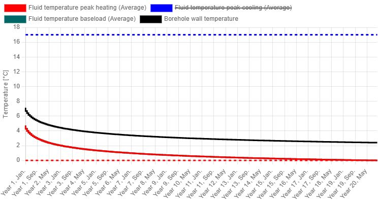
Although this method represents the long-term effects of the borefield fairly well, it does not account for monthly variations, peak loads, or the behaviour in the first year of operation. These elements are introduced in the level 2 methods and beyond.
Level 2 – three-pulse method
The three-pulse method, also known as the ASHRAE sizing method, is the most traditional approach for calculating the required borehole depth. It builds on the level 1 method by adding two additional heat pulses: one to account for the peak power and another for the energy exchanged with the ground during the month in which this peak occurs.
These three pulses, representing the imbalance, the monthly load, and the peak power, collectively capture both the long-term and short-term thermal effects of the borefield, resulting in a relatively accurate estimation of the required borehole depth. A graphical representation of this approach is shown in the figure below.
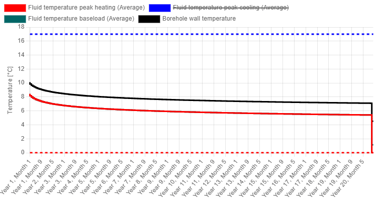
In the figure, the three distinct pulses are clearly visible. First, there is a long-term temperature trend similar to the one produced by the level 1 method, representing the effect of the annual imbalance. Then, a sudden drop appears due to the energy exchanged during the critical month (monthly load), followed by an even sharper drop in fluid temperature caused by the peak extraction event.
This method does not account for monthly variations in the load profile, a level of detail that is introduced in the level 3 sizing method.
Level 3 – monthly resolution
Calculating the required borehole depth with a monthly resolution is the most common approach when using GHEtool Cloud, particularly in cases where only limited data is available. This method includes the same elements as previous levels such as peak powers, long-term ground interaction, and ground properties but also incorporates monthly variations in the load profile.
This results in higher accuracy, as it accounts for seasonal thermal energy storage, meaning the seasonal variation in borehole wall temperatures is now reflected in the sizing. A typical temperature profile calculated with this method shows this seasonal fluctuation clearly.
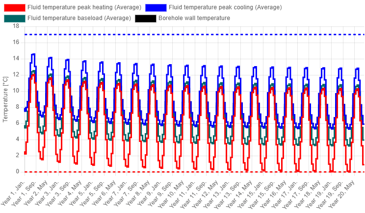
An important parameter in the level 3 method is the duration of the peak power. Depending on the building type and its emission system, this duration typically ranges between 6 and 12 hours, though longer durations are also possible. This assumption, however, is no longer required when moving to a level 4 sizing.
Level 4 – hourly resolution
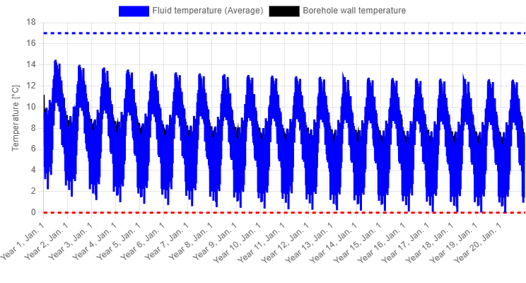
The most advanced method for calculating the required borehole depth is the level 4 method. Unlike the level 3 method, which works with monthly resolution, the level 4 method uses hourly input data. The key advantage of this approach is that the remaining assumption regarding the duration of the peak power is no longer necessary, as this information is directly extracted from the hourly profile itself. When hourly data is available, the level 4 method is the most accurate way to determine the required borehole depth.
Gradient error
Since GHEtool considers, in contrast to other design software, both the maximum and the minimum temperature limit, a so-called ‘gradient error’ can occur quite often, especially in projects with a rather high cooling demand. In this section we’ll discuss in depth where this error comes from and how to overcome it. We’ll do this by first talking about the sizing with a constant ground temperature and afterwards a sizing with a temperature gradient.
Sizing with a constant ground temperature
Imagine that there is no temperature gradient in the ground meaning that, regardless of depth, the undisturbed ground temperature remains constant. When this is the case, the only thing that changes the fluid temperature, is the total borehole length.
Since the gradient error only occurs when there is an issue with the maximum fluid temperature, we’ll only need to consider the injection case. Since the peak injection power remains the same when using the calculate required borehole depth method(as it is determined by the building demand), a greater total borehole length results in a lower specific heat injection rate per metre of borehole, which in turn leads to a lower fluid temperature. This is illustrated in the figure below.
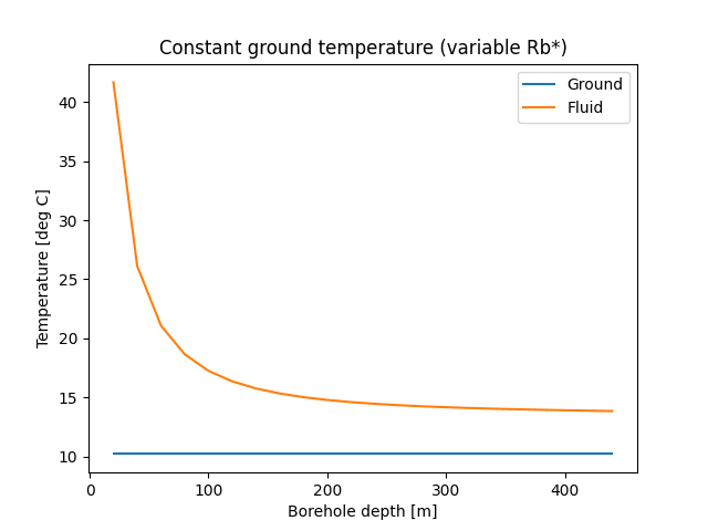
As can be seen in the graph above, which was simulated with a variable effective borehole thermal resistance, the maximum average fluid temperature indeed decreases with increasing depth and converges to a constant difference with the ground temperature. If the final fluid temperature remains below the temperature threshold (for example 17°C), a solution can always be found.
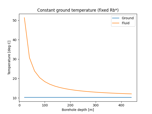
The reason why the profile with the variable borehole resistance is different is because the effective borehole (as discussed in Part 2.2) is also a function of depth and a combination of both the local borehole resistance as well as the internal resistance. Whereas the specific injection power $\dot{q}$ keeps going down with increasing borehole length, the borehole resistance increases, due to the increase in thermal short-circuiting between the downward an upward going flow. Both effects more or less cancel each other out leading to the constant temperature difference.
Sizing with temperature gradient
A more realistic situation is when a ground temperature gradient is present. As discussed in Part 1.3, the ground heats up when you are going down. This means that with increasing the borehole depth, the ground temperature increases. Just like before, with increasing depth, the fluid temperature converges towards a constant difference with the ground temperature, but since this now increases as well with increasing depth, the following ‘combined effect’ is visible.
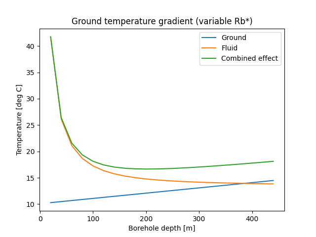
As you can see in the graph, both effects are now combined: there is a sharp decrease in the maximum average fluid temperature at first, followed by a (small) increase over time due to the rising ground temperature with depth. This results in a convex curve for the maximum average fluid temperature (shown as ‘Combined effect’).
If the minimum of this curve lies above the temperature threshold, then there is no mathematical solution to the sizing method, and a gradient error is thrown.
Gradient error
To illustrate this error further, let’s take a look at the figure below, which is a simplified version of the previous graph.

With two boreholes, the maximum average fluid temperature (in this example) is always above the threshold, so no solution can be found where the maximum fluid temperature stays below the set threshold. The only way to resolve this is to increase the number of boreholes, as shown in the graph on the right. Since there are now 50% more boreholes in the borefield, the total borehole length is also 50% more for the same borehole depth (and hence ground temperature). This causes the entire graph to shift downward, resulting in a feasible solution.
Borefields that are limited by the maximum average fluid temperature will therefore always benefit from having more, shallower boreholes rather than fewer, deeper ones.
As could be seen in the figure above (right), there are two solutions that satisfy the threshold temperature, each with a different borehole length. The left solution corresponds to a case where the ground temperature has little influence on the fluid temperature, and the maximum average fluid temperature is mainly determined by the specific heat injection per metre of borehole. The other, right, solution occurs when the ground is already rather warm, but the specific heat injection is relatively low.
Due to the mathematical nature of the problem and the iterative approach, it is not always straightforward to predict which optimum the iterative method will converge to. However, the first one is generally the cheapest due to the lower total borehole length. Therefore, another sizing approach has been developed for GHEtool.

The figure above on the left shows the traditional iterative approach. First, an initial guess is made, after which a new depth is calculated. This process continues until the temperature threshold is reached (or a gradient error is thrown). Depending on your initial guess, load profile, ground parameters, borehole thermal resistance, etc., it is not known a priori which solution the iteration will converge to.
Within GHEtool, we’ve developed a novel sizing method that makes use of the underlying physics of the borefield. Instead of iterating back and forth around a certain optimum, our algorithm starts with the most shallow option and converges towards the first solution, giving you the most affordable borefield.Example in GHEtool Cloud
To illustrate how this method works, let us consider an example in GHEtool, the full detail of which are given in the downloads below.
The project at hand is a case with 4 boreholes, a heating demand of 22 MWh/year with a peak power of 15 kW and a cooling demand of 7.6 MWh/year and a peak power of 10 kW. Using a double U tube, 25 v/v% of MPG and a variable flow rate with a constant temperature difference of 3°C and calculating the required borehole depth, we get the gradient error below.

When the simulation is run again but now with 5 boreholes, a required borehole depth of 116.36 m (so a total borehole length of 577 m) was found and the temperature profile is given below.
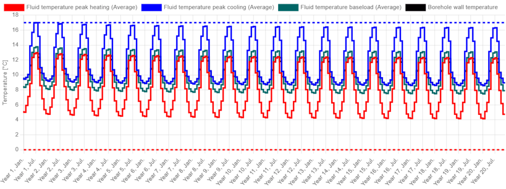
The temperature profile above illustrates why there was a gradient error in the first place. Since the borefield sizing is clearly limited here by the maximum average fluid temperature, the algorithm can get stuck in the downward spiral of drilling deeper to lower the injection per meter borehole, but increasing the ground temperature. Adding another borehole makes the situation feasible.
When we switch to active cooling, the maximum average fluid temperature can be higher meaning that the 4 boreholes are now enough. Running the calculation leads to a required borehole depth of 91.99 m or 364 m in total. The temperature profile is given below where it is visible that the borefield is now limited by the minimum average fluid temperature.

The simulations above were done using the assumption of a homogeneous ground with a thermal conductivity of 2 W/(mK). However, imagine you have actually two ground layers: the first one being a sand layer, up to a depth of 70 m with a conductivity of 2 W/(mK) followed by a clay layer with a worse conductivity of 1 W/(mK).
In this case, using the assumption of a homogeneous ground can lead to wrong results since the calculate required depth algorithm updates the depth thereby changing the ground properties. If the simulation is run again using these two ground layers, a required drilling depth of 96.1 m is found, leading to a total of 380 m, around 5 % more than before.
Conclusion
This chapter described the 5 different levels for borefield sizing, from simple rules of thumb to detailed hourly simulations. However, when both the maximum and minimum fluid temperature are considered, it is possible that this methodology has no answer and a gradient error is returned. This can be overcome by increasing the number of boreholes, as was also shown in an example in GHEtool.
In order to overcome the occurrence of the gradient error, another methodology has been developed to calculate both the required borefield size and depth. This will be discussed in the next chapter.
References
- Peere, W., Picard, D., Cupeiro Figueroa, I., Boydens, W., and Helsen, L. (2021). Validated combined first and last year borefield sizing methodology. In Proceedings of International Building Simulation Conference 2021. Brugge (Belgium), 1-3 September 2021. https://doi.org/10.26868/25222708.2021.30180
- Ahmadfard, M. (2018). A Comprehensive Review of Vertical Ground Heat Exchangers Sizing Models With Suggested Improvements. Thèse de doctorat, École Polytechnique de Montréal. https://publications.polymtl.ca/3034/
Questions
Downloads
- Download GHEtool simulation from this chapter here.